RDP 2007-12: Dynamic Pricing and Imperfect Common Knowledge 4. Price Dynamics
December 2007
- Download the Paper 287KB
This section presents the main results of the paper. By simulating the model described in Section 3, a number of issues are addressed. First, it is demonstrated how the variance of the firm-specific wage-bargaining shock influences the degree of inflation inertia, and that the model can explain the positive coefficient found on lagged inflation in estimates of the hybrid new Keynesian Phillips curve. Second, it is demonstrated that the model can replicate the observed large magnitudes of individual price changes as compared to changes in the aggregate price level, as well as match the observed average duration of individual prices found in the data.
Throughout this section, some of the parameters of the model will be held fixed. These are the persistence of the labour supply shock ρ, the discount factor β, the inverse of the intertemporal elasticity of consumption γ, the curvature of the disutility of supplying labour φ and the parameters in the Taylor-type rule. These will be set as {ρ,β,γ,φ,ϕπ,ϕγ} = {0.9,0.995,2,2,1.5,0.5}. The choice of the exogenous persistence parameter roughly reflects the persistence of various measures of marginal cost (for instance, the labour share in GDP). The precise value of ρ is not important, though some exogenous persistence is necessary to generate interesting results. The parameterisation of the discount factor β at 0.995 reflects that a period in the model should be interpreted as being one month in order to make the assumption that inflation is observed with a one period lag realistic. The Calvo parameter θ should thus be interpreted as the fraction of firms that do not change prices in a given month and, unless otherwise stated, it will be set to θ = 0.9, which implies an average price duration of 10 months. The exact choice of the parameters in the period utility function and the Taylor-type rule (γ, φ, ϕπ and ϕγ), are not crucial for the results below.
The focus in the analysis below is on the role played by the idiosyncratic shocks
to firms' marginal costs. The variance of these shocks relative to the
variance of economy-wide disturbances determines how precise a firm's own
marginal cost is as an indicator of the economy-wide averages. As a matter
of normalisation, the variance of all other shocks are held fixed, as the variance
of the idiosyncratic marginal cost shocks is varied in the exercises below.
The variance of the demand shock  and the variance of the innovation to the persistent labour supply shock component
 are therefore set to unity.
The labour supply shock λt is a compound of two shocks with different persistence.
The technical reason for this set-up is that if it was a process with a single
innovation in each period, the lagged price level would perfectly reveal the
lagged labour supply shock and any information-induced dynamics of inflation
would be short-lived. Since the focus of the paper is the consequences of private
information, rather than imperfect information in general, the variance of
the transitory labour supply shock component  is set to 0.01. This
is small enough to make the effects of firms' confounding persistent and
transitory economy-wide shocks insignificant, but large enough so that lagged
inflation does not completely reveal the persistent labour supply shock component
ξt.
4.1 Inflation Dynamics and the Size of the Idiosyncratic Shocks
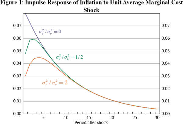
Figure 1 illustrates how the variance  of the idiosyncratic wage bargaining shocks affects the dynamic response of inflation
to a unit shock to the persistent component ξt of the
labour supply shock λt. The blue curve is the response
with the idiosyncratic marginal cost shock variance set to zero. The green
and orange curves are the impulse responses with the idiosyncratic shock variance
set to 1/2 and 2, respectively.

Three things are worth pointing out. First, with a zero idiosyncratic component variance,
the model replicates the full information response, with monotonic convergence
to the mean after the shock. Second, with a non-zero variance of the idiosyncratic
marginal cost component, the response of inflation is hump-shaped, with the
peak of the hump appearing later the larger is the variance  .
Third, the larger this ratio is, the smaller is the first-period impact of
a marginal cost shock and the lower is inflation at the peak. Since the underlying
labour supply shock in all three cases decreases monotonically, and in a shape
identical to the inflation response with a zero variance ratio, the humps must
be driven by the dynamics of the higher-order expectations of average marginal
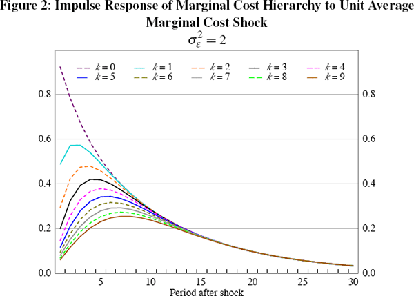
cost. Figure 2 displays the dynamics of the hierarchy of marginal cost expectations
up to the third order, that is,
  , after a unit shock to the persistent component
ξtof the labour supply shock with the variance of the
idiosyncratic marginal cost shock set to
  .
.

Figure 2 shows that the average first-order expectation moves less than the zero-order marginal cost on impact. The idiosyncratic component thus works as ‘noise’ in the filtering problem that smooths out estimates of the innovations in the average marginal cost process. In addition, higher-order estimates move less on impact than first-order estimates. The key to understanding the dynamics of the higher-order estimates is that common knowledge of rationality implies a recursive relationship between orders of expectations. Firms' first-order estimate of average marginal cost is rational given their information set, but they know that due to firms confounding idiosyncratic and economy-wide disturbances, shocks are underestimated on average (that is, average first-order expectations move less than the actual shock). Therefore, for a given change in first-order expectations on impact, second-order expectations move less as firms expect other firms to, on average, underestimate the shock in the impact period. A similar argument applies to third- and higher-order expectations and explains why the response of expected marginal cost in the impact period is decreasing in the order of expectation.
In the model presented here, individual firms have two different types of information: the private observation of its own marginal cost and the public observation of lagged inflation and output. A well-established result from the literature on social learning is that when agents receive both private and public signals, and there are strategic complementarities in actions, agents tend to put too much weight on the public signal relative to its precision, which is often referred to as ‘herding’.[12] Herding slows down the social learning process by making the endogenous signal, that is, the observed aggregate behaviour, less informative about the underlying exogenous shock. Another way to understand the inertia of inflation is thus that firms herd on public signals that are only observable with a lag.
4.2 The Model and Actual Inflation Dynamics
In the preceding sections I presented qualitative evidence in the form of hump-shaped impulse responses on how imperfect common knowledge can introduce inflation inertia. In this section, the question is asked whether the model can account for the observed inflation inertia in US, euro area and Australian data, with quantitatively realistic amounts of information imperfections. This question is pursued by generating data from the simple general equilibrium model and estimating the hybrid new Keynesian Phillips curve
by generalised method of moments (GMM). If the model is the true data-generating process, then the hybrid new Keynesian Phillips curve is of course misspecified. The experiment of interest is thus to check whether the misspecified econometric model (48) applied to the theoretical model would produce results similar to those obtained when the hybrid new Keynesian Phillips curve is estimated on actual data. Galí et al (2005) provide a range of estimates for the US and the euro area, using slightly different choices of instruments and formulations of the orthogonality condition. The estimates of the backward-looking parameter γb ranges from 0.035 to 0.27 for the euro area and from 0.32 to 0.36 for the US. A robust feature across methodologies is that the estimated inflation inertia is lower in the euro area than in the US. Estimating the same equation on Australian data from the post-inflation-targeting period (1993:Q1–2006:Q4) yields backward-looking parameter estimates of between 0.36 and 0.5.
Table 1 displays estimates of the hybrid new Keynesian Phillips curve (48) using simulated data from the model for different ratios of the variance of the bargaining shock over the variance of average marginal cost.[13]
 |
μb | μf | κ |
|---|---|---|---|
| 1/10 | 0.19 | 0.81 | 0.024 |
| 1/2 | 0.34 | 0.66 | 0.013 |
| 1 | 0.41 | 0.59 | 0.010 |
The simulated data was transformed to ‘quarterly’ frequencies by taking three period averages. The orthogonality condition was then estimated by GMM using all available lagged variables, that is, marginal costs, output and inflation rates, as instruments.
Table 1 tells us that the variance of the idiosyncratic bargaining shock only needs to be about 1/2 the size of the variance of the average marginal cost for the model to generate the inflation inertia observed in the US. Quantitative information on the magnitude of unexplained firm-level variations in real wages are hard to come by, but there are some studies where this information can be extracted as a by-product. Martins (2003) investigates the competitiveness of the Portuguese garment industry labour market using yearly data. He finds that between 30 and 40 per cent of average wage variations across firms cannot be explained by labour market conditions, changes in the skills of workers, production techniques or (time dependent) firm-level fixed effects. It is not clear that this is representative of other industries and countries. However, the fact that the model requires a variance ratio of 1/2 to match US inflation inertia cannot be considered conspicuously unrealistic.
4.3 The Model and the Evidence on Individual Price Changes
In addition to matching the observed inertia of aggregate inflation, the model can also reproduce some features of the behaviour of individual goods prices. Two widely cited studies on the frequency of individual good's price changes are Bils and Klenow (2004) on US consumer price data, and that carried out by the Inflation Persistence Network of the central banks within the Eurosystem. The latter is summarised in Alvarez et al (2005). Both of these studies find that prices of individual goods change infrequently, but less so for the US than for the euro area. Bils and Klenow report a median probability of a good changing price in a given month of around 25 per cent. The distribution of the frequencies of price changes is not symmetric and the average price duration therefore differs from the reciprocal of the median frequency. The average duration of prices in the US is around 7 months, rather than (1/0.25) = 4 months. A recent study by Nakamura and Steinsson (2007), using a more detailed data set than Bils and Klenow, finds that the average price duration of consumer prices in the US is between 8 and 11 months for the sample period 1998–2005. Alvarez et al find a median duration of consumer prices in the euro area of about 10 months.
The micro evidence also suggests that individual prices are much more volatile than the aggregate price level. Klenow and Kryvtsov (2005) find that, conditional on a price change occurring, the average absolute individual price change is 8.5 per cent for the US, which is the same number reported by Nakamura and Steinsson (2007). This can be compared with the average absolute monthly change in the US CPI of 0.32 per cent for the period 1981–2005. Average absolute individual price changes are thus about 25 times larger than average absolute aggregate price changes.
The price level is non-stationary in the model of this paper which, together with the Calvo mechanism, prevents an analytical derivation of the absolute average size of individual price changes. What can be done instead is to use the law of motion of the system (34) and the inflation Equation (36) to simulate the model and then compute the average absolute change in both the aggregate price level and of a typical individual good's price. The inflation Equation (36) implies that the price level follows
since πt = pt − pt−1. The optimal reset price of good j in period t is then given by
since  .
It is clear from Equation (51) that increased price stickiness, that is, a
higher θ, will increase the relative size of individual price
changes to aggregate price changes; when fewer firms change prices in a given
period, they have to move by more for a given change in the aggregate price
level to occur. In the model here, the idiosyncratic component affects the
relative size of individual and aggregate price changes through two additional
and distinct channels.
First, there is the direct effect of larger idiosyncratic marginal cost shocks on the magnitude of individual price changes; more volatile individual marginal costs will lead to more volatile individual prices.
Second, the larger is the variance of the idiosyncratic component, the less precise is a firm's own marginal cost as a signal of aggregate marginal cost. As demonstrated above, increasing the variance of the idiosyncratic component leads to more muted responses to aggregate shocks. Since the idiosyncratic shocks cancel out in aggregate, it is only the second indirect effect that affects the aggregate price level. The magnitude of individual price changes relative to aggregate price changes therefore unambiguously increases as the variance of the idiosyncratic component of marginal costs is increased.
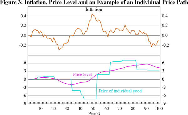
In Figure 3, simulated series of inflation, the aggregate price level and the price of a typical good are plotted. The variance of the idiosyncratic marginal cost shock is set to 1/2 of the variance of average marginal cost. It is clear from the bottom panel of the figure that, conditional on a price change occurring, individual good prices are much more volatile than the aggregate price level.

The aggregate price level path and the path of an individual good's price can be simulated for various ratios of idiosyncratic and economy-wide marginal cost shock variances so as to compute the relative size of the average absolute price changes of an individual good compared to the average absolute aggregate price level changes. The results of this exercise for different degrees of price stickiness are reported in Table 2.
 |
E|Δpt(j)|/E|Δpt| | |
|---|---|---|
| θ = 0.8 | θ = 0.9 | |
| 1/10 | 6.3 | 13.4 |
| 1/2 | 6.6 | 17.5 |
| 1 | 7.1 | 20.4 |
Comparing the two columns to the right in Table 2 tells us that the average magnitude of individual price changes relative to aggregate price changes are significantly larger when the average price duration is 10 months (θ = 0.9) as compared to an average price duration of 5 months (θ = 0.8), suggesting that it may be important to match the frequency of price changes when calibrating models to replicate the observed average price changes of individual goods. With an average price duration of 10 months, the model can match the numbers reported by Klenow and Kryvtsov (2005) and Nakamura and Steinsson (2007) of individual price changes, on average, being 25 times larger than aggregate price changes, by setting the idiosyncratic marginal cost shock variance to be approximately 1.4 times the variance of the economy-wide average marginal cost.


