RDP 2007-05: Labour Force Participation and Household Debt 3. The Modelling Strategies

Using the available HILDA Survey data, we estimate both a cross-section and a panel model for LFP. Within the cross-section framework, we test for the potential endogeneity using an instrumental variables approach.

3.1 Cross-section Model

The relationship between debt and LFP is modelled using cross-section data from the 2002 HILDA Survey, which allows us to make use of the more detailed household balance sheet information collected in that year. The propensity to participate in the labour force is modelled as a function of a vector of Assets, of Debts and of personal and family characteristics, X. As only the outcome of the LFP decision is observed, a latent variable approach is used. The dependent variable, LFP, is defined as 1 if the individual is employed or looking for work in the week prior to the interview and 0 otherwise, and LFP* is the latent variable:

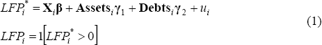
More specifically, the probability of LFP is modelled using a probit specification:

where Φ is the cumulative normal distribution.

Consistent with the literature, we choose a model of individual LFP. The literature often finds more significant effects associated with the decision to work rather than for the decision between positive hours (Heckman 1993). Rather than estimating a model for the household jointly, the labour force status and income of the individual's partner are included as explanatory variables.

Assets may be an important determinant of LFP as they capture a potential wealth effect and may also better capture the effects of non-labour income. In addition, asset holdings may reduce the effect of any credit constraints.

3.2 Accounting for the Potential Endogeneity

The potential endogeneity of debt in the LFP decision, discussed in Section 2.2, is tested using a two-step instrumental variables approach, as suggested by Rivers and Vuong (1988).^[3] Along with Equation (1), the system of equations includes a reduced-form equation for Debts:

Debts are modelled as a function of all of the exogenous variables in Equation (1) and a set of instrumental variables, Z. These instrumental variables, Z, appear in Equation (3) but not Equation (1) and are used to isolate the variation in Debts that is exogenous to LFP. The test developed by Rivers and Vuong will find that debt is endogenous to LFP if u and ν are correlated. The instruments used are discussed in Section 5.2.

The instrumental variables strategy provides a solution to the potential endogeneity if two conditions are satisfied. The first, which can be tested explicitly, is that the instruments must be correlated with Debts. The second condition is that the instruments must not be correlated with u, the error term in Equation (1). In general, this second condition must be maintained by assumption. However, where there are more instruments available than potentially endogenous variables, an overidentification test can be performed to assess whether the instruments are correlated with u.

3.3 Exploiting the Longitudinal Data

A panel model is also estimated using the longitudinal data from the HILDA Survey. These data enable each individual's unobservable and time-invariant characteristics to be controlled for, although the available assets and debt data are less comprehensive than for the cross-section model. Ignoring this unobserved individual heterogeneity can potentially result in biased estimates (Baltagi 2005).

Both a fixed-effects and a random-effects model are used to explicitly account for the longitudinal nature of the data. The model is similar to Equation (1) above but with data available for each individual i over time t:

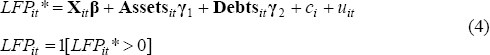
where the individual effect c_i captures the unmeasured characteristics of each individual that are stable over the sample period. These might include risk preferences, attitudes to, and aptitudes for, work, or unobserved permanent components in wages (Chamberlain 1984). Both methodologies, fixed- and random-effects, ‘eliminate’ c_i from the estimating equation and so the potential bias from the unobserved heterogeneity is eliminated. Baltagi (2005) and Wooldridge (2002) each provide a detailed exposition of both methodologies, along with the form for the probability model as per Equation (2).

For the fixed-effects estimation, a logit functional form is assumed and a conditional fixed-effects logit is estimated. By conditioning on X_i, Assets_i, Debts_i and c_i, and by excluding those individuals that are always in or always out of the labour force, β, γ₁ and γ₂ are consistently estimated and the influence of c_i is eliminated.^[4]

For the random-effects model, a probit functional form is used. To consistently estimate β, γ₁ and γ₂, it is assumed that the X_it, Assets_it and Debts_it are independent of C_i, as well as u_it, for all i and t.^[5] Only if this assumption holds is c_i ‘eliminated’ from the estimating equation. It is a strong assumption but can be tested using a Hausman test of the random- and fixed-effects estimates. If the random-effects point estimates are not found to differ from the fixed-effects estimates, random effects is preferred as it is more efficient.

The advantage of fixed-effects estimation is that it produces consistent estimates, and indicates how people change their LFP in response to changes in debt over time. However, only observations on individuals who change labour force status during the sample period can be included in the estimation. As a result, only a sub-sample of less than a quarter of the size of the full sample of women and around 10 per cent of the full sample of men are available for estimation.^[6] In addition, no time-invariant characteristics may be entered in the model.

On the other hand, the random-effects model is favoured because it can be estimated on the full sample, and Baltagi (2005) argues that random-effects is appropriate if the sample is drawn randomly from a large population and is broadly representative. This is the type of sample available from the HILDA Survey. In addition, the random-effects estimates can be easily used to examine the marginal effect of debt on LFP probabilities.

Footnotes

While accumulated assets may be a result of previous labour force activity, it is reasonable to assume that assets are exogenous to current labour force status. In any case, there are no reliable instruments available to test for the endogeneity of assets. [3]

Fixed-effects probits cannot be estimated because a conditional distribution that does not depend on c_i cannot be found (Wooldridge 2002). [4]

That is, . [5]

Tests of the characteristics of these sub-samples show that those who vary their labour force status are quite different from those who remain in or out of the labour force. For example, those women who changed status were more likely to have a partner, young children, less debt or no university education. Men who changed status were less likely to have debt, a partner, university education, English proficiency or be Australian born. [6]