RDP 2002-01: Inflation Targeting and the Inflation Process: Some Lessons from an Open Economy 4. Evidence of Changes in the Inflation Process
January 2002
- Download the Paper 272KB
In order to operate an inflation-targeting regime, and to assess the range of options facing policy-makers, it is crucial to have a reasonable understanding of the inflation process. The policy-maker's desired response to a given shock depends on its most likely effect on inflation, particularly in the medium term, which, in turn, ultimately depends on the behaviour of inflation expectations. An important factor which small open economies have to contend with is that shocks to the exchange rate, which occur frequently and are often large, can have a significant direct effect on the inflation rate. Understanding the link between changes in the exchange rate and inflation is thus particularly important.
Over the latest decade, however, there have been indications that the inflation process in many industrialised countries may have changed. The monetary policy, or inflation, reports of inflation-targeting central banks, for example, allude to a fall in the extent of pass-through of exchange rate shocks to domestic retail prices in several different countries over several different episodes:
Exchange rate passthrough continues to be more muted and diffuse than historical experience would suggest… (Reserve Bank of New Zealand Monetary Policy Statement, March 1999, p 13)
…staff analysis suggested that import prices had fallen by less than was expected given the rise in the exchange rate…In other words, the pass-through from exchange rate appreciation had been unexpectedly weak. [Members concluded that] since the pass-through from the earlier much larger appreciation seemed to be incomplete, there was a good chance that the recent depreciation would have little effect. (Bank of England, ‘Minutes of Monetary Policy Committee Meeting’, 8 and 9 October 1997, p 4)
…the exchange rate normally affects inflation through import prices…In practice, however, the weak krona has not affected either import or consumer prices as much as the Riksbank had anticipated. (Speech by First Deputy Governor Lars Heikensten, Monetary Policy and the Exchange Rate, Riksbank, 19 April 1999)
Import prices have for some time exerted a restraining influence on consumer price inflation. The extent of this effect was unexpected. Historical experience suggested that, given the exchange rate depreciation between mid 1997 and late 1998…some eventual impact in the form of higher import prices at the retail level could be expected. (Reserve Bank of Australia Bulletin, ‘The Economy and Financial Markets’, August 1999, p 32)
This is a possibility that has been raised and explored in a number of papers in recent years.[10]
There have also been suggestions that the inflation process more generally may have changed in recent periods. Taylor (2000) examines data for the US, and finds a reduction in the ‘persistence’ of inflation shocks. That is, he finds that the inflation process in the US is less highly autocorrelated in the 1980s and 1990s than it was in the previous two decades. Taylor argues that the low inflation outcomes of the latest two decades may have caused this reduction in persistence. Kuttner and Posen (1999) also present evidence of a reduction in the persistence of inflation in Canada, the UK and New Zealand in the period since they have been inflation targeting. They argue that this reduction in persistence may reflect the success of the inflation-targeting regime in ‘enhancing public trust of the central bank's long-run target commitment’.
In a recent paper, Andersen and Wascher (2001) take a different perspective. They show that there has been a systematic positive bias to OECD inflation forecasts during the 1990s, and examine whether particular shocks, which have been common across countries, can explain these outcomes. They also explore whether structural changes in the inflation process can be identified. They conclude that there is no systematic explanation across countries for the lower-than-expected inflation outcomes, and the structural changes they find are neither common across countries, nor are they statistically significant.[11]
The Australian experience has been similar to that of many other OECD countries. During the 1990s, inflation was both lower and considerably less variable than would have been predicted at the beginning of the decade, and the response of inflation to exchange rate shocks, in particular, has been considerably more muted. Dwyer and Leong (2001) examine the Australian experience and look for evidence of a structural change in both the inflation process and the process that drives each of the major determinants of inflation. Using recursive estimation techniques, they provide tentative evidence that the speed with which exchange rate changes are passed through to consumer prices has fallen. Although they do not find that this change is statistically significant, they emphasise that the magnitude of the change would be economically significant. They also discuss changes to the wage-setting process in Australia over the last two decades, and argue that these are likely to have dampened the transmission of price shocks to wages and hence reduced the potential for wage/price spirals to develop.
In this part of the paper, we further explore these issues. First, we estimate a simpler, reduced-form price equation for Australia in an attempt to summarise the dynamics of the combined price and wage setting processes.[12] Similar equations are estimated for New Zealand, Canada, the UK and the US by way of comparison. Unlike earlier studies, however, we then use rolling regressions with a 10-year window to gauge the changes in these processes that are taking place. Although rolling regressions provide less efficient coefficient estimates than recursive regressions, they can also provide a clearer indication of structural changes as they are occurring. Our focus is as much on whether these changes would be of economic significance as whether we can reject the statistical hypothesis of no structural change at conventional levels of significance.
We derive the equation we estimate from the following two reduced-form relationships:
where π is the log difference of the aggregate price level, πe is expected inflation, πm is the log difference of import prices and y is the log of output relative to potential. π* is discussed below.
The first equation is a Phillips curve, where inflation outcomes depend on expected inflation, growth in real import prices (a measure of the real exchange rate), the output gap and the change in the output gap. The last term reflects the fact that in the Australian data, the speed at which the output gap is being closed, as well as its level, is typically important.
The second equation describes the process by which inflation expectations are formed. Some proportion (Σβk) of inflation expectations is formed in a backward-looking manner, and the rest (1−Σβk) is anchored at some constant rate of inflation, π*, which we will call the perceived inflation target. Over time, it is therefore possible that both the perceived inflation target π* and the extent to which inflation expectations are linked to the target rate (1−Σβk) may change, and movements in these two can be distinguished from each other. So if Σβk = 1, inflation expectations are entirely backward-looking, while if Σβk = 0, they are completely anchored to the target, π*.[13]
Substituting (6) into (5), and assuming k = 2, we have the equation that we estimate:
from which individual parameter estimates of the short-run elasticities of inflation with respect to import prices and the output gap, as well as the extent to which expectations are backward-looking (Σβk = δ1+δ2+δ3) and the perceived inflation target (π* = δ0/(1−δ1−δ2−δ3)) can be calculated.
Before we proceed to examine the results, a couple of caveats. The model we are using to capture inflation expectations includes a backward-looking part and an anchored part. This is incomplete, since it does not explicitly include an alternative forward-looking indicator of inflation expectations. One justification for using such a simple model is that in Australia's case, at least, indicators of forward-looking inflation expectations are quite poor, and seem to be quite well explained by an anchor and the recent inflation experience.[14]
Second, the constant term (δ0) in the above equation, and the way in which it changes over time, could reflect several factors in addition to those outlined above. Mismeasurement of the true output gap, for example, would affect the estimate of the constant: if the true level of potential output of the economy were underestimated, the constant (and the implied estimates of the perceived inflation target) would be biased downwards. If the degree of mismeasurement of the output gap changed over time, this could thus explain variations over time in the estimates of the constant. The existence of other sources of structural change that are not captured in this very simple model would also affect the constant term, as would mis-specification more generally. We are thus inclined to interpret any of the results pertaining to the constant term, and hence the estimates of the perceived target rate of inflation, as indicative of the changes that may be taking place, rather than being definitive evidence for them.
4.1 Estimation Results
Equation (3) is estimated for each country over the period from 1983:Q1 to 2000:Q2 using quarterly data. The dependent variable is underlying inflation in Australia's case, and either a measure of core inflation or the first difference of the private consumption deflator for each of the other countries.[15] The lag length of the output gap and import price terms were chosen for each country to best fit the data over the full sample period. The full sample estimates of these regressions are presented in Table 1.
| Coefficient estimates on: | Constant | πt−1 | πt−2 |  |
yt−j | Δt−k | Adj R2 | SE | LM test(1st to 4th) | Chow test(a) |
|---|---|---|---|---|---|---|---|---|---|---|
| Australia | 0.001 (1.6) |
0.408 (3.8) |
0.459 (4.6) |
0.025 (2.4) |
0.048 (2.6) |
0.144 (3.2) |
0.842 |
0.003 |
0.268 |
0.031 |
| New Zealand | 0.001 (1.1) |
0.418 (3.4) |
0.396 (3.3) |
0.063 (2.2) |
0.079 (1.4) |
0.303 (3.3) |
0.641 |
0.007 |
0.210 |
0.001 |
| Canada | 0.003 (2.9) |
0.327 (2.9) |
0.297 (2.8) |
0.010 (0.3) |
0.055 (1.7) |
0.211 (2.6) |
0.332 |
0.004 |
0.513 |
0.020 |
| UK | 0.004 (3.2) |
0.333 (2.9) |
0.282 (2.6) |
0.040 (2.2) |
0.096 (2.9) |
0.143 (1.9) |
0.517 |
0.003 |
0.045 |
0.003 |
| US | 0.002 (2.4) |
0.456 (3.1) |
0.246 (2.0) |
−0.013 (−0.6) |
0.030 (1.1) |
0.068 (1.0) |
0.353 |
0.003 |
0.013 |
0.069 |
|
Notes: The equations were estimated using the following specifications: |
||||||||||
Over the full sample, this very parsimonious model does quite a good job of capturing the inflation process. In Australia's case the equation explains 85 per cent of the variation in quarterly inflation, which is very close to the explanatory power of more fully elaborated models of inflation estimated on the Australian data.[16] In Australia's case, the coefficients on the explanatory variables have the expected sign and are significant. They imply that a 10 per cent shock to import prices would lead to a 0.6 per cent increase in the price level over the following year, and a 1 per cent increase after two years. A 1 percentage point fall in the output gap for one year would lead to a 0.5 per cent fall in inflation over the first year and 0.3 per cent over the second year.
For the other countries, these equations also perform quite well, explaining between 35 and 65 per cent of the variation in quarterly inflation over the full sample. For the NZ, UK and Canadian data, the coefficient estimates are generally of the expected sign and significant. In the case of the US, both the import price term and the output gap terms are insignificant. Across all equations, the coefficient estimates are of similar orders of magnitude.
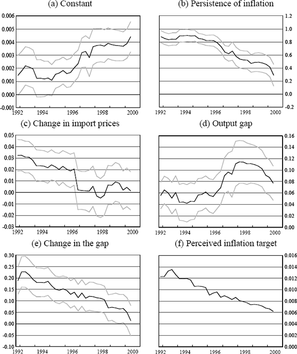
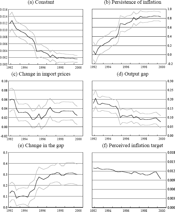
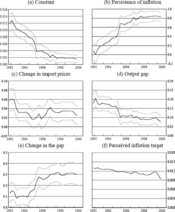
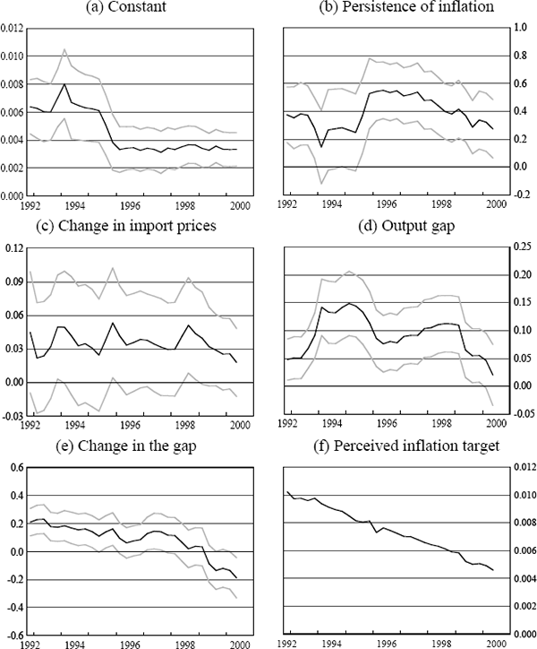
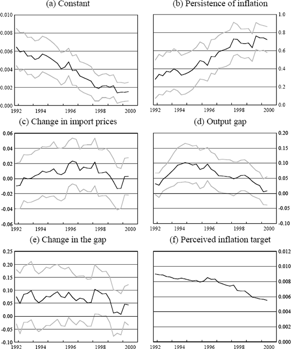
Figures 3 to 7 show rolling regression estimates using the above specifications for each country. In each case, the window is 10-years wide. So, for example, the first point on each of these figures illustrates the coefficient estimates from the equations that were estimated using data from March 1983 to December 1992, and the last point illustrates estimates from regressions taken from September 1990 to June 2000. One-standard error bands around each estimate are also presented.
Notes:
Specification as in Table 1. Grey lines are 1-standard error bands. Persistence of
inflation is (δ1+δ2+δ3).
Perceived inflation target is 
Note: See Figure 3
Note: See Figure 3
Note: See Figure 3
Note: See Figure 3
For Australia (Figure 3), the results point to quite a substantial change in the inflation process over the last two decades. We will discuss each of the coefficient estimates in turn.
First, we focus on the response of inflation to shocks to import prices. Figure 3(c) shows rolling regression estimates of the coefficient on import prices in these inflation equations. It shows that import prices had a significant effect on inflation in the early part of the sample, but they have had no systematic effect on inflation outcomes since around 1987. In other words, once the large depreciation of the exchange rate in the mid 1980s is excluded from the estimation period, inflation has been much less sensitive to exchange rate developments. This could reflect a change in the price-setting process of either importers or retailers, or it could reflect a non-linearity in the effect of exchange rate developments on inflation outcomes. It could also reflect the fact that the depreciation of the mid 1980s, as well as being large, was widely perceived as being permanent, because it coincided with a period in which commodity prices had fallen particularly sharply and the current account deficit had increased markedly. The depreciation was thus widely interpreted as being necessary to assist the Australian economy adjust to these developments. In most other episodes, in contrast, it was much less clear whether exchange rate changes were likely to be permanent or temporary.
Note that the models we are estimating are designed primarily to capture the short-run dynamics of the inflation process. It would thus be unwise to use them to draw conclusions about changes in the extent of exchange rate pass-through over a long horizon. It is possible, for example, that the long-run relationship between imported prices and consumer prices has changed little, but pass-through has become more protracted.[17] In an inflation-targeting framework, however, this change still implies that a given shock to the exchange rate would require less of a policy adjustment.
Interestingly, the lack of response of inflation to exchange rate developments is also evident in the New Zealand data (Figure 4(c), again especially after the first few years of the sample are excluded) while for Canada (Figure 6(c)) and the UK (Figure 5(c)), these coefficient estimates have stayed roughly stable over the sample period. So while the recent experience in Australia and New Zealand would suggest that inflation has become less sensitive to exchange rate movements, this has not been a common experience for these other open, inflation-targeting countries, all of which have recorded low inflation outcomes in recent periods.
The coefficient on the output gap in the Australian equation has varied somewhat over the sample period (Figure 3(d)), and has been both higher and statistically more significant in the second half of the sample. On the other hand, the coefficient on the change in the output gap (Figure 3(e)) (i.e., the indication that there are ‘speed limits’ to growth) has drifted down over the period and has been insignificant in regressions starting from around 1987. The latter trend would be consistent with the increasing flexibility of both product and labour markets in Australia.
For the other countries, estimates of the coefficient on the change in the output gap have also varied quite a lot over time, and in the case of New Zealand, for example, as in Australia, the change in the output gap appears to have been a much more significant explanator of inflation developments earlier in the sample than it has been more recently. The estimated coefficients on the level of the output gap have been roughly stable in the case of the UK and Canada, while for the US, the coefficient has drifted down towards zero as the sample increasingly includes the 1990s.
We now turn to estimates of the degree of autocorrelation, or persistence, in the inflation process. In the model outlined above, these estimates correspond to estimates of the degree to which inflation expectations can be characterised as being backward-looking. For Australia, Figure 3(b) suggests that over the last two decades, the inflation process has become markedly less autocorrelated. These estimates could be interpreted as implying that during the 1980s, inflation expectations were based almost exclusively on past inflation developments, while during the 1990s, close to 70 per cent of inflation expectations can be characterised as being tied to a target rate of inflation. This result support the Kuttner and Posen (1999) hypothesis that the adoption of inflation targeting has increased the capacity of the central bank to manage inflation, by reducing the propagation of inflation shocks. The results could also, however, be interpreted as providing support for Taylor's (2000) hypothesis that the persistence of inflation shocks decreases in a low-inflation environment.
Turning to the results for the other countries, however, qualifies these conclusions (Figures 4(b), 5(b), 6(b), 7(b)). Only in the case of Australia and New Zealand has there been a clear decline in the persistence of inflation over the period, although in both of these cases it has been quite sharp. In the UK and the US, by contrast, the degree of persistence appears to have increased quite markedly and monotonically from the 1980s to the 1990s, while in Canada it has remained roughly unchanged. The results for the US are counter to those presented in Taylor (2000); these rolling regression estimates suggest that conclusions about persistence are quite sensitive to the time period chosen.
There is no obvious explanation for the diversity of these outcomes across countries. All of the countries we are considering (other than the US) became inflation targeters in the early 1990s, and all have achieved very low inflation outcomes during the latest decade. In the case of Australia and New Zealand, it is plausible that other structural changes in the economy, in particular the deregulation of the labour market, could be responsible for a large part of the reduction in the degree of persistence in the inflation process. As pointed out in Dwyer and Leong (2001), in 1985 around 80 per cent of wages in Australia were indexed and by 1990 this proportion had fallen to less than 10 per cent. Similar (and even more far-reaching) changes to the industrial relations system occurred in New Zealand. But this can't explain why, over the 1990s, the persistence of inflation was so much lower in Australia and New Zealand than in the US and the UK, given the flexibility of the latter countries' product and labour markets. More generally, the wide variation in these estimates over time and across countries suggests that any conclusions drawn from these sorts of reduced-form price equations may not be particularly robust.
Overall, the results in this section of the paper suggest that there may well have been structural changes in the inflation process in each of these countries between the 1980s and the 1990s. Chow tests of structural change, presented in Table 1, support this conclusion at a 10 per cent level for the US and at a 5 per cent level for each of the other countries.[18]
Like Andersen and Wascher (2001), however, we find that the structural changes that have occurred in the inflation processes have differed quite a lot across the countries considered and it is hard to attribute these changes to any specific global phenomenon. In particular, it seems unlikely that increased credibility can convincingly be argued to have driven the reduction in inflation persistence found for Australia and New Zealand given the other countries' results. As a result, it will be important to remain on the lookout for further changes to the inflation process.
Footnotes
See, for example, Cunningham and Haldane (1999), Dwyer and Leong (2001), and McCarthy (1999). McCarthy (1999) finds that for the nine OECD countries he examines, pass-through is considerably lower over 1983–1998 than it was over the full sample period (1976–1998), although he claims that these differences are probably statistically insignificant. [10]
Their paper examines forecasts and developments in eight OECD countries: US, Japan, UK, Canada, Australia, Spain, Sweden and Switzerland. It compares the behaviour of inflation during the 1990s with that of the previous three decades. [11]
These equations are similar to those estimated in Andersen and Wascher (2001). [12]
These two equations imply that in the short run there is a trade-off between output and inflation, but in the long run, provided inflation expectations eventually adjust one-for-one with actual inflation there will be no trade-off. If Σβk = 1 this will always be the case; if Σβk<1, it thus requires that π* eventually converges on the actual inflation rate. [13]
See Footnote 5. [14]
See Appendix B for further details. [15]
In Beechey et al (2000), an error correction model for quarterly changes in the acquisitions CPI is estimated; it explains around 90 per cent of the variation in quarterly inflation. This model has a richer dynamic structure, and incorporates unit labour costs and oil prices as well as the explanators included above. [16]
Gruen and Leong (2001) present evidence which supports this conclusion. [17]
Table 1 reports tests for a structural break at March 1992, but the results were not particularly sensitive to the break point. For simplicity, a common break point was chosen across countries at a time that coincided roughly with the beginning of the low-inflation episode for most of these countries. These results are in contrast to those presented in Andersen and Wascher (2001), although in that paper, the authors were testing whether the inflation process in the whole of the 1990s (including the disinflationary period at the beginning of the decade) was significantly different from the behaviour of inflation during the previous three decades. Beechey et al (2000) also do not find statistically significant evidence of a structural break in the Australian inflation process in the error correction model they estimate. That equation, however, includes unit labour costs as an explanator, where the equation estimated above is a reduced-form price equation. Our tests for structural change are thus implicitly tests for structural change in either the price or wage-setting process. [18]


