RDP 2001-08: City Sizes, Housing Costs, and Wealth Appendix A: A Model of City Formation and Dwelling Prices

Cities

There are N cities, with city i located at position l_i having population P_i and share of total population p_i ≡ P_i/P where P ≡ Σ_iP_i. The cities are randomly placed around a circle, implying 0 ≤ l_i < 2π. This simplifies the analysis while at the same time being a reasonable approximation of Australia's geography. The distance between cities is therefore:

For the purpose of this paper, we assume that city locations are fixed. However, it may be possible to use models such as Krugman's (1996) to extend our model to allow city locations to be endogenous.We leave this task to future research.

Firms

There are two types of firm, local and country-wide.^[21] Firms are of equal size, with the number and share of local firms in city i denoted F_i and fi, and similarly C_i and c_i for national (country-wide) firms. We denote the share of national firms in total firms as β.

Local firms (f-firms) sell only into the city market they are in, and compete only with other firms in that city. Therefore their location decisions are driven by the relative size (population share) of each city, and also influenced by the number of local firms already in that city. The probability that a new local firm will choose to locate in city i is assumed to be proportional to:

where α is an index of the intensity of competition or substitutability of the new firms' output with the output of firms already in city i.

If α = 0 (local firms are monopolists selling differentiated goods), the model reduces to a standard Bose-Einstein occupancy problem where growth in F_i is roughly proportionate to city i's population (Hill 1974). If α > 0, growth in F_i is less than proportionate to P_i when f_i > p_i and more than proportionate when f_i < p_i. In the limit, f_i will converge to p_i and growth in the number of firms will display the random proportionate growth required for Gibrat's Law to hold. Therefore, a does not affect the limiting behaviour of the model, but will help determine its speed of convergence.

National firms (c-firms) sell into the entire national market and are not affected by the location decisions of their competitors. New firms of this type locate so as to minimise transport costs, which are assumed to be proportional to distance, and land rent, which is assumed to be proportional to average dwelling price, h_i. The choice for these national firms is to choose city i, where i minimises

The parameter θ represents transport costs per unit distance. Since d(i,i)=0, (A4) implies that most firms of this type will locate in the largest city, unless the largest city is a long way from the rest of the population or land prices are particularly high. We can interpret local firms as those in service and retail industries such as restaurants, doctors, supermarkets and so on, while national firms are likely to be in industries such as finance or manufacturing.

Housing costs

Households prefer to minimise commuting time and will therefore pay a premium to live closer to the city centre. Assuming commuting times are linear in distance, and that the premium paid for location is proportional to commuting time, then house prices h vary linearly with distance from the centre, r. This is similar to the early models of intra-city housing costs (Mills 1967; Muth 1969), although in those models prices decline at a decreasing rate with distance from the centre.

In (A5), R is the maximum extent of the city, and the price of housing at the fringe, H = h(R), is set to zero for simplicity. Housing costs that are declining in distance from the centre fit in with the von-Thünen-Mills models of land rent and allocation around a central place (Mills 1967). If the city is circular, its area – equivalently, population or number of dwellings – is P_i = πR². There are 2πr dwellings at radius r. Therefore the city's average housing price, h_i varies with the square root of its population.

This functional form depends on the assumption of a fixed floor for housing prices; prices at the very fringe of the city do not depend on the size of the city. It is also possible that commuting times will vary more than proportionately with distance from the centre, due to congestion. Alternatively, the development of edge cities and increasing prevalence of employment opportunities in the suburbs could mean that congestion costs rise less than proportionately with population (Krugman 1995). However, this will not reverse the central result that average housing prices are higher in larger cities, and that national average housing prices are higher when the population is concentrated in a few centres. In the simulations below, we define h_i as , effectively setting the scaling factor ψ to .

Household location decisions

We assume a city's attractiveness to households depends on three factors: the availability of jobs, the absolute population of the city and the average level of housing costs. We measure the availability of jobs by ((1 − β)f_i + β c_i)/p_i. The direct inclusion of city populations is intended to account for the observed wage premium seen in larger cities (Glaeser and Maré 2001). This may reflect either that search costs are lower in larger labour markets, or that larger markets allow for greater specialisation, which raises wages. In addition, larger cities have more diverse industrial structures and thus may be attractive locations to a wider range of workers (Gabaix 1999b).

Housing costs work against these forces encouraging greater agglomeration. Although there may be other disadvantages to living in large cities, such as congestion, pollution and crime, we take housing costs as a proxy for all of these costs, given that they are monotonic in city population. Since the attractiveness of a city, u(·) represents the utility it offers to its residents, we assume that it has a fairly standard functional form, the Cobb-Douglas function. This ensures declining marginal utility of absolute city size.

Following Gabaix (1999a), we assume that in each period t, g_t P new households are born and δP households die; the death rate δ is constant across time and across cities.^[22] Total births nationwide are random, with the growth rate g_t distributed lognormally with mean γ and a variance that depends on σ². The allocation of new households to cities is determined by the attractiveness of that city relative to the national average of all cities. This relative attractiveness is scaled so that their weighted sum equals one. Suppressing the time subscripts, we have:

We define the birth rate in city i, g_it as a lognormal random variable with common variance σ² and a mean that is scaled by the relative attractiveness of that city in that period. The scaling factor used in the definition of relative attractiveness (A8) ensures that the mean growth rate for the total population equals γ.

Importantly, we do not assume that all (new) households move to whichever is the most attractive city, as this would result in the system having unstable dynamics. Depending on the relative importance of housing costs versus employment opportunities, either the largest city would then increase without limit while the other cities fade away at rate δ, or the smallest, cheapest, city would attract all the new population and become large. If the smallest city attracts the population, it is then no longer the most attractive city, and the city that had previously been the second-smallest attracts all the new population in the following period. The functional forms for the utility and housing-price relations used here result in the net effect of rising population on its relative attractiveness varying with . If 1−λ is very different from µ/2, the (unbounded) city population effect dominates the effect of job availability in the long run. This does not materially distort the simulation results presented below, as the net effect of city population remains fairly small for the range of populations considered.

By contrast, allowing random growth in all cities captures the reality of the process of birth or household formation, while allowing households to respond to economic forces by having some change location. Random growth with a mean depending on economic factors effectively captures moving costs – it is not always advantageous to move to the most attractive city – and unobserved heterogeneity – not everyone will want to move even if it would benefit the median new household. Alternatively, these costs and individual variation could be modelled, but only by adding many free parameters and functional forms without much theoretical guidance to pin them down. In our view, this would add complexity to the model without adding much explanatory power.

One final adjustment is required to prevent city populations from being zero. The actual increase in population in each city is defined as:

where ε is a small positive number which we set equal to 1. Gabaix (1999b) showed that random proportionate growth with a lower bound on population, which he termed a Kesten process, will generate Zipf's Law in the upper tail of a size distribution.

Simulation results

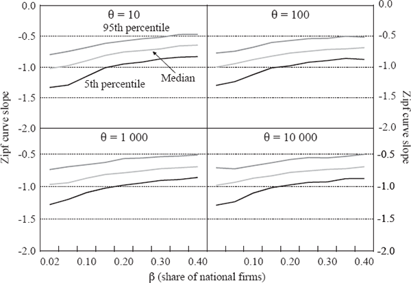
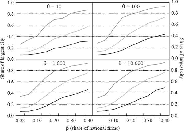
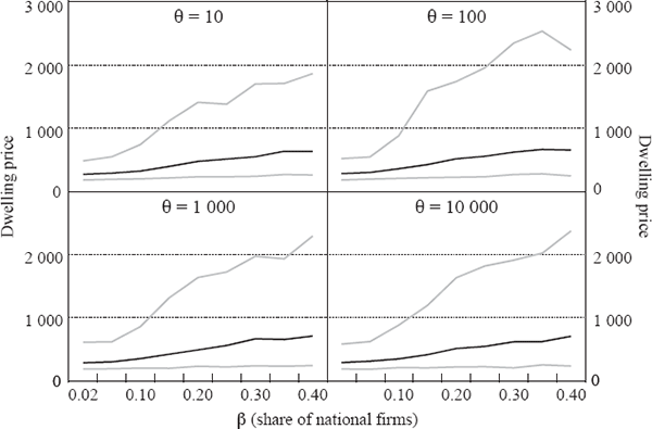
The results in this Appendix are based on an extensive exploration of the model for a range of parameters. For each pair of values for the parameters β and θ, we conducted 500 simulations, each of 500 periods for a country of 100 cities. The α parameter does not affect the long-run results, so we set it to 0.5 throughout. The mean birth rate γ was set to 0.03 and the death rate δ to 0.02. The parameters in the household utility function are λ = 0.9 and µ = 0.15, so large cities are on balance more attractive than smaller ones even when the labour market in each city is in equilibrium. Similar results are obtained within a significant neighbourhood of these parameter values. The figures below show the median final-period outcome and the 5th and 95th percentile of those 500 cases, for dwelling prices, the largest city's share of the total population and the slope of the ‘Zipf curve’, or log rank-log size relationship, for the top 50 cities. We find that the rank-size relationship tends to flatten out after this point. This is in line with the finding that random growth generates Zipf's Law in the upper tail of the distribution, but not necessarily for the whole sample (Gabaix 1999b; Hill 1974); a simple Kesten process as in Equation (A10), where g_it is a random variable drawn from a common distribution, will generate a Zipf curve with a linear segment covering about half to two-thirds of the sample.

If the share of national firms in the economy β is small, say, less than about 0.05, our model generates rank-size curves roughly consistent with Zipf's Law (Figure A1). As β rises, the simulations tend to generate flatter Zipf curves, with slopes around 0.5–0.7. With β above about 0.4, a primate city is almost guaranteed (Figure A2).

As expected, increasing importance of national firms (β) and transport costs (θ) both result in the largest city having a larger share of total population. Flatter Zipf curves and large primate cities imply higher national average dwelling prices (Figure A3). This seems in line with Australia's situation: countries with relatively small populations (high β) spread over large distances (high θ) will have more concentrated populations and higher average housing costs than countries without these characteristics.

The model we have used is not a complete model of city formation. In particular, we have left many stylised features of the economics of cities as exogenous factors, such as the wage premium paid in large cities. The location decisions of households and firms are assumed to depend only on current-period payoffs. In a more complex model, agents would be forward-looking instead of myopic, but as Neary (2001) argues, and Baldwin (1999) demonstrates for the core-periphery model, this added complexity does not affect the model's comparative-statics predictions. We also generated the higher housing costs in larger cities observed in Section 2.3 by geographic construction; a more sophisticated model would allow residents to respond to housing costs by endogenously adjusting the size and quality of new dwellings. Although random birth of households is biologically justifiable, the random allocation of local firms (f-firms) is less justifiable on economic grounds. Recent research has developed models that can explain these features as endogenous outcomes of microeconomic behaviour, at the cost of considerable extra complexity and computational burden (Axtell and Florida 2001). Nonetheless, our model illustrates that a few simple variations on a random-growth model can generate rank-size distributions that match the data for a range of countries reasonably well.

Footnotes

This distinction is a variant of the approach taken by the existing literature. For instance, Krugman (1996) assumes two sectors: a geographically immobile sector (agriculture) and an increasing returns, monopolistically competitive, geographically mobile sector (manufacturing). [21]

We assume that each household contains one person. [22]