RDP 2001-01: The Decline in Australian Output Volatility 4. The Structural VAR

I use three variables in the VAR: output growth, the unemployment rate and the terms of trade (TOT). These variables are chosen to use the same variables as Blanchard and Quah (1989) augmented with the TOT to reflect the fact that Australia is a much more open economy than the US. I will not be imposing any restrictions on the model above those required to achieve identification. As such the details of the individual equations are relatively unimportant. The VAR methodology specifically allows the data to suggest the best model.

Underlying the VAR we can think of three orthogonal structural shocks ε^s, ε^d, ε^TOT. These are i.i.d. shocks to supply (productivity), demand and the TOT. ε^s is a productivity shock that may have permanent effects on output while ε^d is a demand shock that is constrained to have no long-run effect on output. ε^TOT is a shock to the level of the TOT which is also constrained to have no long-run effect on output.

The exact variables used (i.e. whether in levels or differences) are discussed in the next section. For the time being I will just describe the relation between output, unemployment and the terms of trade. Suppose that the relation between x = (y,ue,TOT)′ can be characterised by the structural equations:

where:

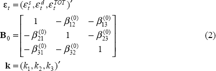
and B_s is a general (3×3) matrix. This can be rewritten in more standard VAR form by premultiplying both sides by .

where:

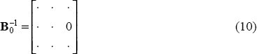
Identification of the structural parameters requires identification of the parameters of B₀. Given knowledge of B₀ the remaining B_s can be identified from the reduced form VAR parameters. There are six free parameters in B₀ so six restrictions are needed to identify them. The first three restrictions come from assuming that the underlying shocks are mutually orthogonal and, thus, that their covariances are zero. This is implemented through a number of nonlinear restrictions on B₀. In particular:

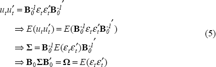
and we require that Ω_ij=0 for i ≠ j. A consistent estimate of Σ is obtained from the reduced form VAR residuals.

The remaining three restrictions are generated from economic argument in the manner of Blanchard and Quah (1989). The first two are that demand shocks and terms of trade shocks have no long-run effect on the level or growth rate of output.

The long-run restrictions are now widely used but still controversial. Much of the justification for their use has already been given previously (see, for example, Blanchard and Quah (1989)). Notwithstanding this, I present some reasons why terms of trade and demand shocks may not have any long-run effect on output. As argued in Blanchard and Quah (1989) there may be reasons to think that demand shocks can have long-run effects on output. However, the size of these effects is likely to be very small compared to that of supply disturbances. As such, the identification that demand shocks have no long-run effects is ‘almost correct’.

It is possible to imagine two forces driving the terms of trade: long-term structural changes in the composition of imports and exports and fluctuations in the prices of a relatively stable basket of imports and exports. In the latter case there should be no significant long-run effect on output. In the former case you might well expect these changes to affect output. However, in these cases the shocks are more reflective of output and demand changes than terms of trade fluctuations. These shocks will appear in the terms of trade but are probably better identified with domestic factors such as demand or supply. The identification strategy used explicitly rules out long-run effect from the terms of trade and thereby focuses on the short to medium-term price fluctuations in the terms of trade. The longer-term changes are associated with supply shocks. I will return to this consideration when the final results are interpreted. Notwithstanding this, it is possible to change the identifying assumptions and relax the assumption that terms of trade shocks have no long-run effect. This is done at the end of the section.

The long-run restrictions are implemented as follows:

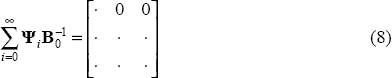
It is possible to write the reduced form VAR in MA(∞) form

If xⁱ is included in the VAR in differences then the long-run effect of a shock in ε^j on the level of xⁱ is the row i, column j element of

where Ψ₀ = I.^[4] Thus, the two long-run restrictions are imposed as:

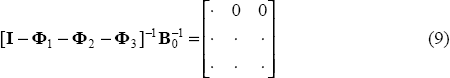
In practice, we can use the VAR representation to impose the long-run restriction. If, for example, we have estimated a VAR(3) model, the long-run cumulative effect of an innovation in u_t on x_t is given by [I −Φ₁ −Φ₂ −Φ₃]⁻¹.^[5] That is, 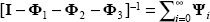. Thus, the long-run restriction on the effect of ε^j on x_t can be imposed as:

The remaining restriction imposed is that the terms of trade has no contemporaneous effect on unemployment. This captures the fact that there are lags in the effect of the terms of trade on the economy. This is the simplest to implement as it amounts to requiring that:^[6]

Thus, these restrictions guarantee identification of the structural model from the reduced form estimation.

The robustness of these results was tested by varying the set of restrictions among a wider set of alternatives. The results are relatively insensitive to the particular restrictions chosen. When alternative contemporaneous restrictions are imposed the results are generally the same. Restricting the TOT to have no contemporaneous effect on output or restricting the TOT to have no contemporaneous response to productivity or demand shocks did not alter the results. Furthermore, there was little change in the results from allowing the TOT to have some long-run effect on output.^[7] In this case the estimated long-run effect on output was very close to zero. This suggests that long-run changes in the composition of imports and exports that would have long-run effects on the terms of trade and output are better captured by the model as supply shocks than terms of trade shocks.

4.1 Separating Structure and Shocks

Identifying whether the reduction in output volatility is due to the structure of the economy or the shocks hitting it is a central objective of this paper. This section outlines the strategy that will be used to make this identification.

Following the discussion in Section 3, structural change is identified as a change in the coefficients of the structural VAR while a change in shocks is a change in the variance of the structural errors. Thus, changes in Ω are changes in shocks and changes in B₀,…,B_p are structural changes or, more correctly, changes in the propagation mechanism.

For example, volatility in output could emerge due to an increase in the size of demand shocks or through a change in the propagation of those same demand shocks through the economy. In practice many changes are occurring at once. Policy rules change as well as interest rate shocks. Demand shocks change at the same time as supply shocks. The propagation of demand shocks through the economy, perhaps through greater economic integration, may be more or less damped.

Structurally similar models (those with similar parameters B₀,…,B_p) should react similarly to given shocks while there should be a different response when the same shocks are applied to structurally dissimilar models. A useful metric for evaluating the volatility of a model is the forecast error variance (FEV) of output at some given horizon. In the tables below I will consider separately the effect of the structure on the FEV and the size of the structural shocks. The second is easy to see as it is just given by the matrix Ω. Thus, we can see what has happened to the individual shocks, whether their variance has risen or fallen. The first is slightly more complicated. Nonetheless, identifying the effect of the structure on the FEV requires only a simple modification of the information contained in standard variance decompositions.

The formula for the contribution of the j^th orthogonalised innovation to the mean squared error (MSE) of the s-period forecast is:

where a_j is the j^th column of the matrix and Var(ε_jt) is the variance of the j^th structural shock. In a variance decomposition this is normally divided by the total MSE to give the relative contribution of each orthogonal component. Instead I will focus on the portion in brackets – the structural part. I look at the relative sensitivity of each model to a unit variance structural shock.^[8] Of themselves these responses are not informative, however, by looking at them relative to other periods we can see whether one model is more or less sensitive to particular shocks. Thus, if a given shock in one model leads to a higher overall MSE then we would say that that model is more sensitive to that particular structural shock. If a particular structure is more sensitive to all shocks we can clearly say that it is a less stable structure. Unfortunately, we are unlikely to get a complete ordering of structures on the basis of this observation. What we will get, however, is an indication of which shocks a particular period is most sensitive to.

If a more complete ranking is desired a natural one to consider is given by the following procedure. Consider subjecting one system to the shocks from another system. If the overall FEV is higher in the second system we might conclude that it is less resilient to the kind of shocks that occur in the first system. This uses the relative variances of shocks as the method of weighting the model sensitivities. While still arbitrary, this method provides an easily interpretable result.

Specifically, it can tell how well the 1990s, say, would have reacted to the shocks experienced in the 1970s. If the overall FEV is lower in the 1990s when subjected to the shocks of the 1970s we would say that the 1990s were a more stable system.

Footnotes

This will be the case in the implementation of this paper. In the event that the variables were entered into the VAR in levels the appropriate restriction is that the row i, column j element of is zero. [4]

See Hamilton (1994, p 20) for the presentation of the univariate case. The vector case is a simple generalisation of this. [5]

It makes no difference whether the variable is expressed in levels or differences for this restriction. [6]

To ensure identification, another contemporaneous restriction on the TOT or unemployment is used instead. For example, one set tested consisted of the restrictions: demand shocks have no long-run effect on output, the terms of trade shock has no contemporaneous effect on unemployment and the terms of trade shock has no contemporaneous effect on output. [7]

Although any size would do, as all that is necessary is that Var(ε _jt) be equal for all the structures being evaluated. [8]