RDP 9612: External Influences on Output: An Industry Analysis 3. A Closer Look at Sectoral Links
December 1996
- Download the Paper 182KB
Correlation and graphical analysis provides a useful first pass at assessing whether there are sectoral output links between Australia and the United States, but it tells little about the dynamics and form of the relationship, and it does not control for other effects. Accordingly, we estimate an unrestricted error-correction model of the relationship of domestic sectoral output with US sectoral output, the rest of domestic aggregate output and the rest of aggregate US output:
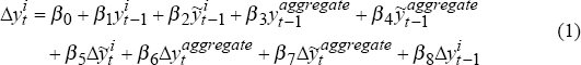
where y is output, the superscript i represents the sector, the tilde denotes the foreign sector, aggregate indicates total output less the sector under consideration and β1<0.[2] Table 2 presents the preferred specification.[3] The equations are estimated in system form using the seemingly unrelated regression (SURE) technique. As outlined in Appendix B, there is considerable correlation between the error terms of these equations at both the one and two-digit levels when they are estimated by OLS. SURE estimation uses the correlation between the error terms of each equation to increase the precision of the coefficient estimates (although if any equation is misspecified all estimates may be inconsistent). The OLS results are also presented in Appendix B. The estimates are less precise but the overall story is qualitatively similar.
| Constant β0 |
Sector adjustment β1 |
US sector adjustment β2 |
Aggregate adjustment β3 |
US aggregate adjustment β4 |
US sector impact β5 |
Aggregate impact β6 |
US aggregate impact β7 |
Lag sector impact β8 |
 |
|
|---|---|---|---|---|---|---|---|---|---|---|
| Total GDP(P) | 1.72** (0.51) | −0.74** (0.19) | 0.92** (0.23) | – | – | 0.54** (0.19) | – | – | – | 0.62 |
| Agriculture | 1.65** (0.69) | −0.91*** (0.13) | – | – | 0.83*** (0.14) | – | – | 1.31*** (0.36) | 0.37*** (0.09) | 0.57 |
| Mining | −8.08*** (1.05) | −1.26*** (0.12) | 0.60*** (0.18) | – | 2.08*** (0.23) | 0.26*** (0.10) | – | 1.23*** (0.31) | – | 0.41 |
| Manufacturing | 3.10** (0.57) | −0.51*** (0.07) | 0.37*** (0.05) | – | – | 0.19*** (0.06) | 0.71*** (0.16) | – | – | 0.73 |
| Food | 2.27*** (0.87) | −0.54*** (0.12) | – | – | 0.34*** (0.10) | – | – | – | – | 0.17 |
| Textiles | 0.94 (1.33) | −0.54*** (0.12) | – | – | 0.33* (0.21) | – | 1.42** (0.63) | – | – | 0.16 |
| Clothing | 8.09*** (0.94) | −0.49*** (0.06) | – | −0.35*** (0.05) | – | 0.57*** (0.09) | 1.03*** (0.26) | – | – | 0.62 |
| Wood & furn. | 3.08*** (0.55) | −0.52*** (0.10) | 0.29*** (0.11) | – | – | 0.22** (0.10) | 2.21*** (0.47) | – | – | 0.48 |
| Paper | 1.65*** (0.39) | −0.32*** (0.06) | 0.27*** (0.10) | – | – | – | 1.88*** (0.31) | – | – | 0.52 |
| Chemicals | 2.39*** (0.50) | −0.43*** (0.07) | 0.28*** (0.04) | – | – | 0.06*** (0.03) | – | – | – | 0.43 |
| Non-met min. | 1.96* (1.06) | −0.67*** (0.08) | 0.25*** (0.06) | 0.20** (0.09) | – | – | 1.85*** (0.49) | – | – | 0.54 |
| Basic metals | −2.30** (0.94) | −0.61*** (0.11) | 0.23*** (0.05) | 0.53*** (0.11) | – | 0.35*** (0.05) | – | – | – | 0.48 |
| Fabr'd met. | 0.12 (0.46) | −0.43*** (0.05) | 0.83*** (0.13) | – | – | – | 2.00*** (0.26) | 1.27*** (0.27) | – | 0.78 |
| Trans. equip. | 15.24*** (1.77) | −1.64*** (0.19) | −0.23*** (0.07) | – | – | – | – | – | 0.94*** (0.13) | 0.53 |
| Other mach. | 5.11*** (0.63) | −0.87*** (0.10) | 0.45*** (0.08) | – | – | 0.45*** (0.10) | – | – | 0.63*** (0.09) | 0.59 |
| Misc manuf. | 3.42*** (0.69) | −0.54*** (0.11) | 0.31*** (0.08) | – | – | 0.48*** (0.06) | – | – | – | 0.63 |
| Utilities | −1.09*** (0.37) | −0.27*** (0.04) | – | 0.28*** (0.06) | – | – | 0.49*** (0.09) | – | – | 0.73 |
| Construction | 2.31*** (0.58) | −0.50*** (0.07) | – | 0.21*** (0.05) | – | – | 1.99*** (0.23) | – | 0.34*** (0.05) | 0.83 |
| Wholesale | 2.22*** (0.83) | −0.46*** (0.14) | – | 0.20*** (0.07) | – | – | 1.38*** (0.27) | – | – | 0.67 |
| Retail | −0.80* (0.45) | −0.77*** (0.09) | – | 0.70*** (0.09) | – | 0.29*** (0.07) | 0.81*** (0.17) | – | – | 0.52 |
| Tran & storage | −4.50*** (0.77) | −1.18*** (0.14) | 0.31*** (0.06) | 1.13*** (0.15) | – | – | 0.99*** (0.14) | – | – | 0.77 |
| Rail | −5.05*** (1.51) | −0.66*** (0.18) | – | 0.77*** (0.22) | – | – | 1.69*** (0.40) | – | – | 0.55 |
| Water | −1.78** (0.86) | −0.76*** (0.20) | – | 0.58*** (0.15) | – | – | 1.08*** (0.39) | – | – | 0.45 |
| Air | 2.28** (0.99) | −0.45** (0.19) | 0.41*** (0.16) | – | – | – | – | – | – | 0.24 |
| Road | −7.47*** (1.11) | −1.40*** (0.18) | – | 1.60*** (0.22) | – | – | 1.05*** (0.21) | 0.63*** (0.22) | – | 0.81 |
| Communic'ns | −0.27** (0.10) | 0.14*** (0.05) | −0.18** (0.07) | – | – | – | 0.46*** (0.15) | – | – | 0.27 |
| Finance | −0.52 (0.40) | −0.26*** (0.06) | – | – | 0.40*** (0.11) | – | 0.60*** (0.18) | 0.53*** (0.14) | 0.68*** (0.05) | 0.75 |
| Recreation & pers. services | −1.72*** (0.23) | −1.25 *** (0.011) | – | 1.08*** (0.09) | – | 0.13*** (0.05) | 0.51*** (0.07) | 0.42*** (0.11) | – | 0.74 |
|
Note: *, ** and *** denote significance at the 10%, 5% and 1% levels, respectively, using the standard t-distribution. |
||||||||||
The long-run impact of a change in foreign output on domestic output is estimated as −β2/β1. A 1 per cent rise in US GDP(P) leads to a 1¼ per cent rise in Australian GDP(P), similar to the coefficient estimated by Gruen and Shuetrim (1994). This coefficient varies between sectors. It is considerably higher in fabricated metals and finance, indicating that growth in these sectors is strong relative to the United States. The final column gives the explanatory power of the equation.[4]
The estimation procedure isolates the influence of foreign sectoral effects and domestic and foreign aggregate demand effects on domestic sectoral output. Moreover, it identifies whether these effects are ‘fundamental’ or long run, as indicated by an error-correction/cointegration relationship between them and domestic sectoral output, or are simply transitory, as indicated by short-run dynamics. Columns 2 to 5 indicate long-run relationships, while columns 6 to 9 indicate short-run dynamics.
Consider, first, foreign effects. Taken overall, developments in the United States are relevant to assessing the prospects for Australian sectoral output. Indeed, after controlling for the effects of domestic demand, about two-thirds of Australian sectoral output has some direct relationship with US output. This connection occurs in a number of forms:
- there are long-run cross-country sectoral linkages, notably in mining, air transport and, in particular, manufacturing. In manufacturing, the long-run sectoral links arise in the production of wood products, paper-related products, chemicals, non-metal minerals, basic metals, fabricated metals, other machinery and miscellaneous manufactures. These sectors comprise about 20 per cent of private-sector output;
- there are long-run cross-country aggregate linkages, by which output in the agriculture, mining and finance sectors and the food and clothing sub-sectors is tied in the long run to aggregate US output. These sectors account for about 30 per cent of private-sector output; and
- there are short run, transitory effects of changes in sectoral or aggregate US output on particular industries, including mining, retail trade, finance, recreation services and various manufacturing sub-sectors. These sectors comprise a little less than two-thirds of private-sector output.
The sectors for which developments in the United States are not important in the long run are usually the ones where domestic aggregate demand is important. So, for example, domestic influences dominate in utilities, construction, wholesale and retail trade, transport and storage (apart from air transport), communications and recreation. There is, naturally enough, also a degree of overlap between domestic and foreign effects in some sectors. For non-metallic minerals and basic metals, both foreign and domestic demand are key long-run determinants of production. For textiles, clothing, wood, paper and fabricated metals production, domestic demand boosts sectoral output in the short run, and the domestic aggregate output impact multipliers are relatively large. Production in most manufacturing sub-sectors can be characterised as being linked to the corresponding US sector in the long run, but substantially affected by domestic aggregate demand in the short run.
What, then, are the distinguishing features of the sectors that are linked to the corresponding US sector? Consider some institutional features, like foreign ownership, export orientation and import competition. Foreign ownership may be relevant if the transmission of technology, human capital and knowledge of market trends is important. Export ratios may contain information about the strength of foreign demand for domestic goods and the importance of foreign preference and technology shocks. Import shares may contain information about the forces of competition in a sector. Thus, these institutional factors may affect the speed of diffusion and the correlation of output changes between countries.
It is difficult to test the hypothesis about the importance of foreign ownership, since information is scant, but Table 3 presents some statistics on foreign ownership by industry. The sectors where US sectoral output links exist are italicised. Columns 1 to 3 present 1982/83 estimates of the foreign, joint and domestic control of industry; column 4 presents the share of foreign investment by sector at June 1983, while columns 5 and 6 present the sectoral levels of foreign investment at June 1994 as a share of total foreign investment and of the sectoral capital stock respectively.[5] Foreign ownership in Australian investment flows in the mid 1980s was relatively high in the finance and property sector and the manufacturing sector – particularly in chemicals, basic metals and transport equipment. The level of foreign investment in finance and property, wholesale trade, mining and manufacturing – in this case, in food, paper, basic metals and transport equipment – is high relative to estimates of the capital stock in those sectors.
| Industry | Capital expenditure 1982/83 foreign control (Share of
total) 1 |
Capital expenditure 1982/83 joint control (Share of total) 2 |
Capital expenditure 1982/83 local control (Share of total) 3 |
Level of foreign investment June 1983 (Share of total) 4 |
Level of foreign investment June 1994 (Share of total) 5 |
Level of foreign investment June 1994 (Per cent of capital
stock) 6 |
Export share 7 |
Import share 8 |
|---|---|---|---|---|---|---|---|---|
| Agriculture | – | – | – | 0.8 | 0.6 | – | 20.8 | 1.9 |
| Mining | 33.6 | 10.8 | 55.5 | 21.0 | 10.7 | 91 | 46.8 | 4.6 |
| Manufacturing | 42.1 | 13.7 | 44.1 | 21.8 | 18.9 | 92 | 10.2 | 20.9 |
| Food | 26.0 | 4.1 | 69.9 | 16.7 | 25.0 | 138 | 16.9 | 5.3 |
| Textiles, clothing etc | 32.1 | 0.1 | 67.9 | 2.3 | 1.3 | 32 | 6.9 | 18.8 |
| Paper, printing | 17.1 | – | 83.0 | 3.0 | 19.0 | 174 | 1.5 | 14.2 |
| Chemicals | 87.5 | – | 12.5 | 12.0 | 8.9 | 66 | 5.7 | 19.4 |
| Basic metals | 76.2 | – | 23.8 | 33.5 | 19.9 | 101 | 38.2 | 10.4 |
| Fabricated metals | 35.0 | 0.8 | 64.2 | 3.4 | 2.2 | 18 | 6.2 | 11.4 |
| Transport equipment | 85.0 | – | 15.0 | 8.6 | 4.2 | 100 | 5.9 | 35.8 |
| Other manufacturing | 18.9 | 2.3 | 78.8 | 10.6 | 5.2 | 87 | 4.5 | 45.4 |
| Misc manufacturing | – | – | – | 3.4 | 13.4 | – | – | – |
| Finance, property & services | 25.7 | 9.5 | 64.8 | 16.0 | 39.4 | 181 | 2.3 | 3.2 |
| Utilities | 0.7 | – | 99.1 | 6.2 | 1.0 | 4 | 0.1 | 0.1 |
| Wholesale trade | 44.6 | 0.2 | 55.3 | {14.2 | 6.9 | 89 | 9.3 | 0.0 |
| Retail trade | 14.5 | – | 85.5 | {14.2 | 1.5 | 26 | 0.0 | 0.0 |
| Transport and storage | 6.7 | 0.4 | 93.0 | 3.8 | 2.5 | 45 | 22.0 | 8.4 |
| Other non-manufacturing | 6.9 | 0.6 | 92.5 | 15.1 | 18.0 | – | – | – |
| Total | 29.9 | 9.1 | 61.0 | 100.0 | 100.0 | 82 | – | – |
Source: Columns 1 to 3 are from Table 3, ABS Cat. No. 5333.0 (naturalised firms are categorised as joint control); column 4 is from Table 27 of ABS Cat. No. 5305.0 1987/88; columns 5 and 6 are from Table 12, ABS Cat. No. 5306.0; data sources for capital stock, export and import shares are provided in Appendix A. |
||||||||
But the proposition that foreign linkages are related to the foreign penetration of the sector does not appear to be supported by these data.[6] Chemicals and paper production both have strong links with US output, for example, but their foreign ownership ratios were very different in the mid 1980s. Similarly, foreign ownership in the transport equipment sub-sector is high, but there is no obvious relationship with US output, despite the fact that the United States is the largest foreign investor in the transport equipment sector in Australia. Foreign penetration of the food sector has increased, and the level of foreign investment is relatively high to the capital stock, but food production is influenced only by the state of domestic demand.
Nor does the external openness of the sector, as measured by industrial export, import or trade shares, seem to be generally important. Columns 7 and 8 in Table 3 measure the proportion of exports and imports in the sector relative to output. But there is no apparent relationship between openness in trade and the existence of sectoral output links with the United States. For example, both basic and fabricated metals have a strong relationship with the corresponding US sectors, but their export intensities are very different.
At least with the data used in this paper, it does not seem that institutional features like foreign ownership or trade openness are relevant to the existence of a long-run or ‘equilibrium’ connection between Australian and US industrial outputs. (This does not mean that the relevance of these features would not be clear at a more microeconomic level.) The explanation of the relationship may lie more with the nature of the industries themselves. The obvious distinction is the difference between goods and services: the output of services is generally dominated by local conditions, while the production of goods is related to both domestic and overseas conditions. Air transport, for example, is the only service sector sensitive to the corresponding US sector in the long run. But all the other sectors for which there is a long-run US connection are in traded goods. These are mining and manufacturing.
While there is a long and short-run link between Australian and US mining outputs, the coefficients on both long and short-run aggregate US output are significantly larger, suggesting that aggregate external developments are the key in this sector. The aggregate effects are also important for agriculture, although cross-country sectoral links are not evident for that sector. For both of these sectors, real prices are set in world markets, and so the value of production is closely tied to world conditions. Since the United States is the largest economy, and in many ways the engine of world economic growth, the value of production is tied to US demand. This seems to be the case even though Australia's resource endowments differ from those of the United States.
The sectoral link is particularly extensive in manufacturing, and it seems to lie with particular sorts of goods. The connections, for example, tend to be in sectors engaged in the production of chemicals, machinery, metals and paper, rather than simply transformed, non-durable consumable goods like food, textiles and clothing. The latter, like services, seem to be produced for the domestic market, and are largely unrelated to sectoral conditions in the United States (although food and textiles are affected by US aggregate demand). Clothing and textiles have also been among the most highly protected sectors in Australia, skewing the market to import substitution and domestic demand. The key distinguishing feature of the first group of goods is that their production is subject to continuing and substantial technological change. For example, research and development, which are indicative of innovation and growth, tend to be highest in sectors like machinery, chemicals and pharmaceuticals.[7] Of course, the technology of food and clothing production has changed over time, but probably not by as much as in chemicals, machinery and metals. Moreover, the transport connection arises only in the air sub-sector, which is the transport sub-sector in which change and the diffusion of technology has been most rapid. Major technological innovations in that and other industries, for example, have led to a rapid expansion of air services and the general use of air freight worldwide. Overall, when the corresponding US sector is important, aggregate US output is not. And these links dominate the long-run behaviour of the domestic sector, such that innovations in the corresponding US sector have permanent, long-lived effects on the corresponding domestic sector. Put together, this leads to the conjecture that the links with US industrial output are driven, by and large, by technological innovations on the supply side. As the production frontier moves out and as innovation in goods takes place, changes in the United States and elsewhere are transferred to Australia. It is striking that the results are so strong when there are limited observations.
The two exceptions to this are domestic output of transport equipment and communications, which have rapidly changing technology, but are not associated with US developments. But there may be special reasons for this. The communications sector in Australia, for example, has grown much more rapidly than in the United States since the mid 1980s, probably due to catch-up after liberalisation. This makes it hard to identify a simple linear relationship with the US sector. Transport equipment, however, has been static and the correlation with US production may have been affected by changing tariff rates in Australia, and a hefty fall and restructuring in domestic US production in the late 1970s associated with the oil price shocks of 1973 and 1979.
The coefficient of adjustment to the long run is about 0.5 for most manufacturing sub-sectors, indicating that half the adjustment occurs after one year and that three-quarters of the adjustment occurs after two years. Changes in production are transmitted within a matter of two to three years. This speed of adjustment ‘makes sense’ relative to other ‘linked’ sectors. For example, adjustment in air transport, the other sector for which there is a long-run inter-sectoral link, is very similar to that of manufacturing. Furthermore, the adjustment in manufacturing is substantially slower than in agriculture or mining – US aggregate demand is central in both of these sectors, and adjustment is completed within a year. The result that it takes a couple of years for developments in US manufacturing to be fully passed through into Australian manufacturing fits in with the general view that the transmission of technology occurs relatively slowly (Costello 1993, p. 216). US studies indicate that the diffusion of knowledge about new products and production processes to rivals is fairly rapid, with the bulk of the spread complete within a year or so (Mansfield 1996, p. 119).
This raises the question of why there is a persistent gap in productivity levels between the United States and elsewhere in the face of continuing technological transfer. In other words, if technology and market trends are being continually transferred, why is Australian manufacturing productivity still only half that of the United States? It is not the case that productivity is higher in the industries where the corresponding sectoral output in the United States is the key driving force. According to Prasada Rao et al. (1995, p. 139), for example, productivity is lower in machinery sub-sectors, paper and wood products than in clothing or food. The sectors where the link with the corresponding US sector is important tend to be those with the lowest productivity relative to the United States. The oddity is probably explained by the nature of the production processes in the two countries (Ergas and Wright 1994). The United States, for example, is the world's largest economy, and this gives it special inherent advantages in economies of scale and market contestability and competition. It also has a labour market which is more flexible and adaptable. The capital stock in Australia may also be older than that in the United States, since updating of plant and equipment occurs less frequently.
Footnotes
The results are the same when aggregate output is defined as total output inclusive of the relevant sector. [2]
The distribution of the lagged-level terms in Equation (1) lies between the Dickey-Fuller (1981) distribution and the standard t distribution (Kremers, Ericsson and Dolado 1992). The standard t distribution is the benchmark for statistical significance in Table 2. The 10 per cent, 5 per cent and 1 per cent Dickey-Fuller significance levels for 25 observations (which is seven more than we have) are 4.12, 5.18 and 7.88, respectively. Generally speaking, when levels variables are significant in an equation, they are also significant at these much higher cut-off points, even at the 1 per cent level. The distribution of the dynamics terms follows the standard t distribution. [3]
When the marginal statistical significance of the equation is above 10 per cent, which roughly corresponds to an R-bar-squared less than about 0.25, we treat the outcome as a ‘non-result’. [4]
The 1982/83 data may be outdated now, but they are around the middle of our sampling period, 1977 to 1993, and so are relevant to the analysis. [5]
This also holds at a more technical level of analysis. We estimated linear probability, logit and probit models with the foreign penetration ratios presented in columns 1, 5 and 6 of Table 3 as independent variables, but the results were always statistically insignificant. The dependent variable was defined as ‘1’ when there was a long-run (or long-run and short-run) relationship between domestic sectoral output and US sectoral output, and ‘0’ otherwise. We also included other variables, such as the export, import and trade ratios of the industrial sector, but also with no success. A casual look at the data suggests that these tests are unlikely to be successful. One problem with the tests is the small number of observations. [6]
For example, in 1986–87, R&D was 3.3 per cent of value-added in transport equipment, 4.5 per cent in other machinery and 2.9 per cent in chemicals, well above the manufacturing average of 1.5 per cent (Bureau of Industry Economics 1990, p. 88). [7]