RDP 9301: The Response of Australian Stock, Foreign Exchange and Bond Markets to Foreign Asset Returns and Volatilities 2. Stock Price Volatilities and Correlations
March 1993
- Download the Paper 128KB
Figures 1 through 6 picture the monthly (end-of-month series) stock price indices and estimated Schwert volatilities for six countries: Australia, Germany, Japan (Nikkei index), Singapore, United Kingdom (Financial Times) and the United States (Dow Jones).
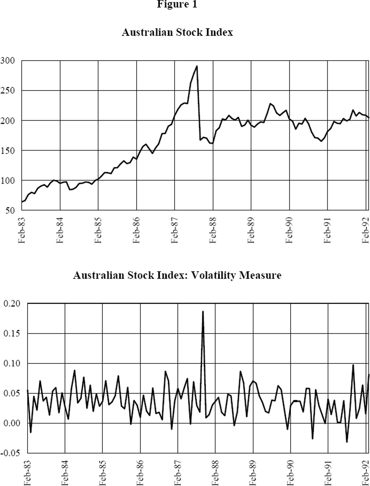
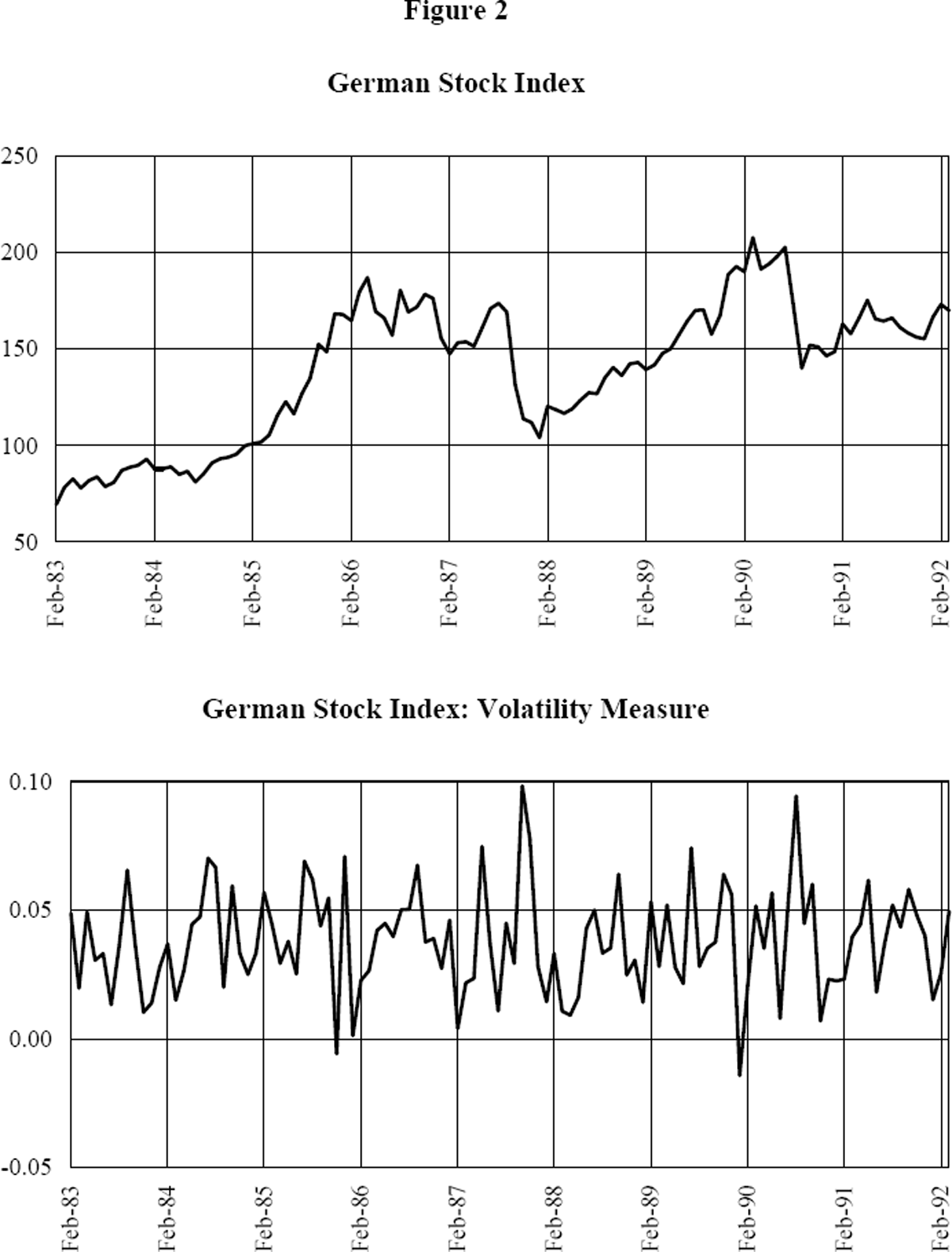
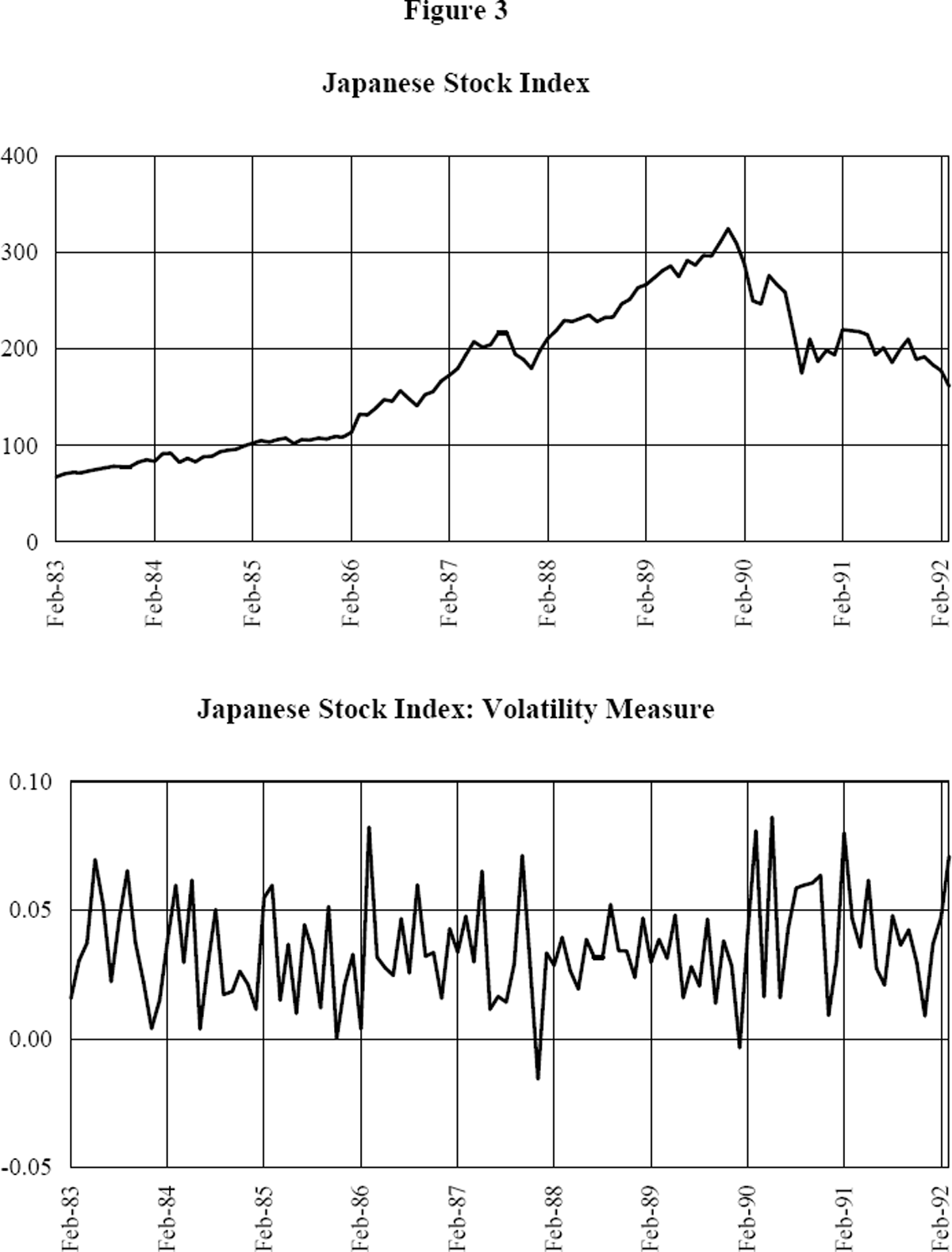
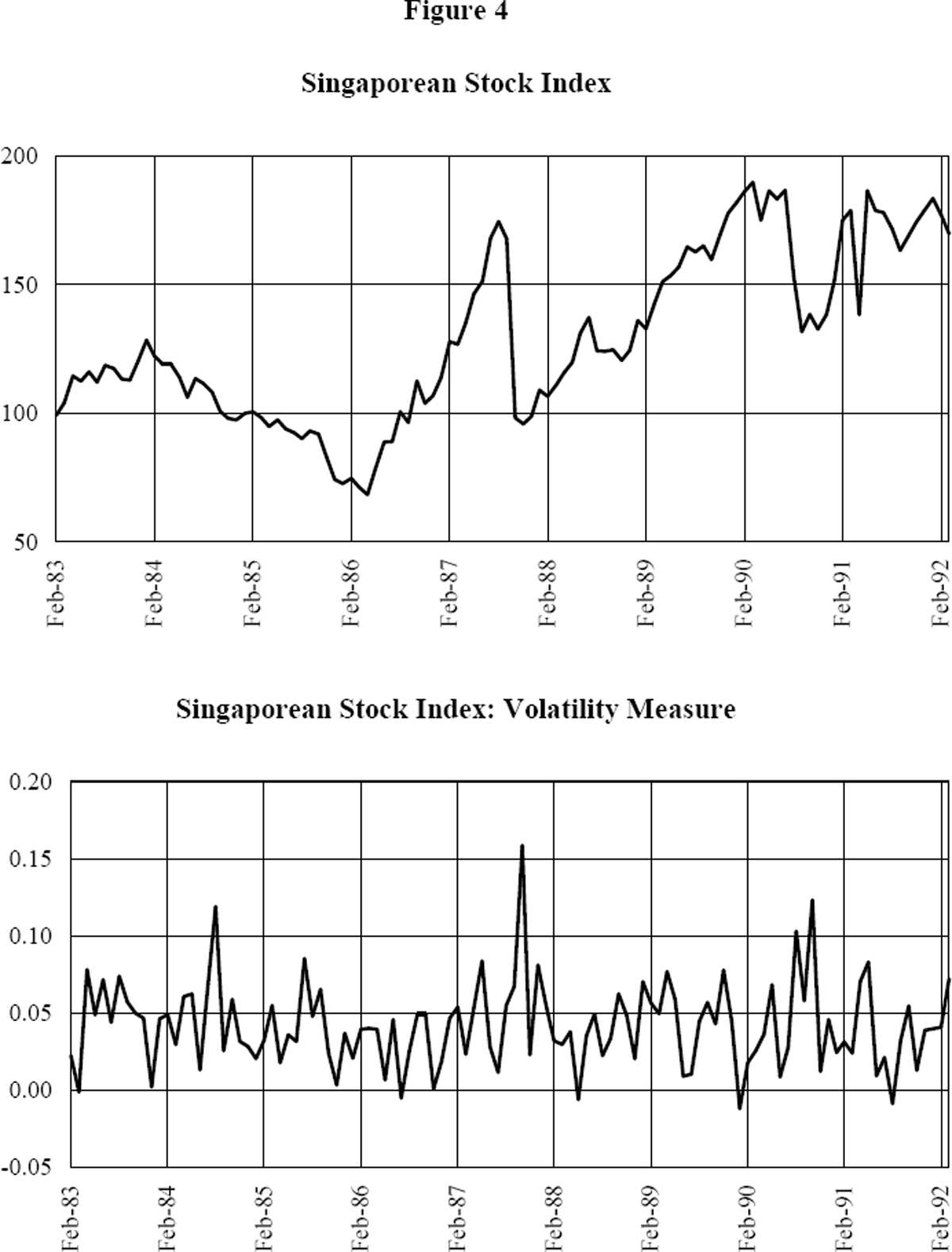
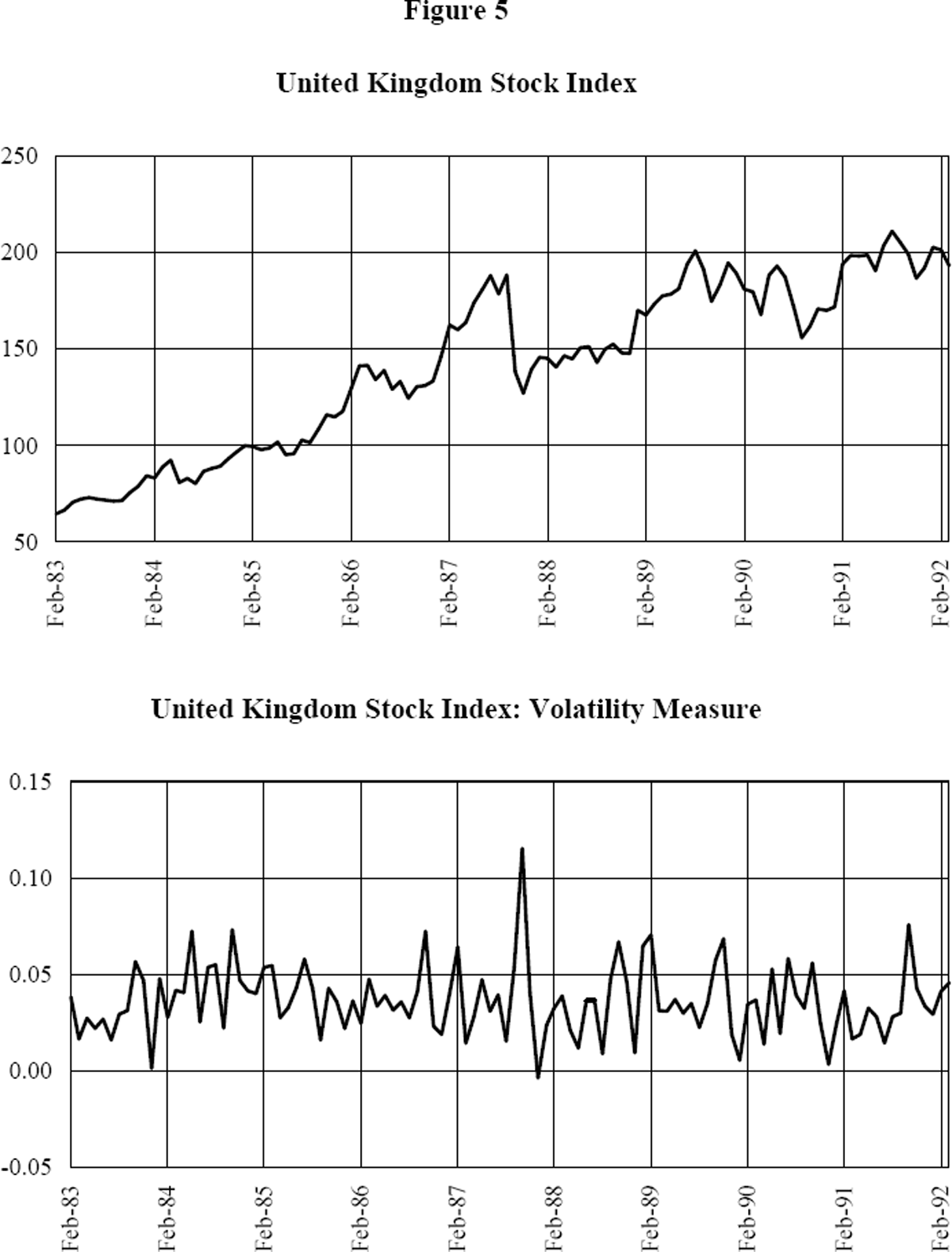
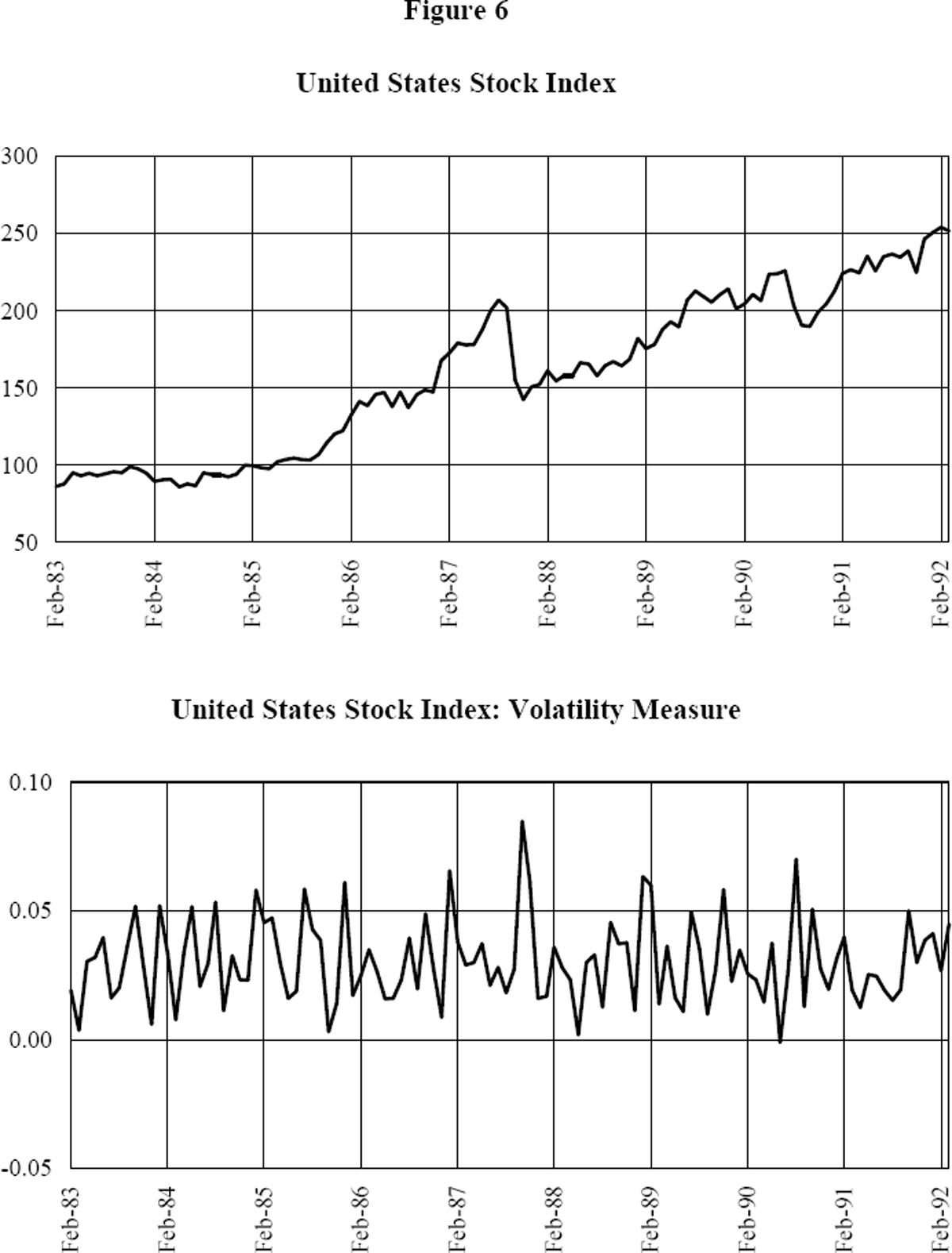
For computing the volatility indices, all data were transformed into logarithmic values and first-differenced. The sample runs from the beginning of 1982 through March 1992. The end-of month data are normalised with January 31, 1985 set at 100[4].
All the figures show breaks in the stock price series at the time of the October 1987 crash. The ‘Black Monday’ (or ‘Black Tuesday’) crash appears as a sharper break in Australia, Singapore, the UK and the US than in Germany and Japan. The Nikkei index did plunge, but several years later, and the fall was less sharp than the break in Australia or Singapore.
The volatility measures appear to oscillate around a band close to .05, with very few departures, except on Black Monday/Tuesday, 1987. At this time, the volatility measure increased almost four-fold in Australia, three-fold in Singapore, and twofold in the United Kingdom. Our results concur with Kupiec that there is no obvious trend toward increasing volatility in the 1980s.
2.1. Contemporaneous Correlations
The estimated correlation coefficients of the volatilities appear in Table I, Panel A. What is surprising is the low correlation of Australian stock price volatility with volatility of the Nikkei index. The three highest correlations, in descending order, are with the UK Financial Times index, the Singapore index, and the US Dow Jones index. The correlation of the UK index with the Australian index is higher than the correlation of the UK index with the Dow Jones index.
| Aust | Germ | Nikkei | Sing | UK | DJ | |
|---|---|---|---|---|---|---|
| Aust | 1.00 | |||||
| Germ | 0.31 | 1.00 | ||||
| Jap | 0.27 | 0.38 | 1.00 | |||
| Sing | 0.58 | 0.51 | 0.37 | 1.00 | ||
| UK | 0.68 | 0.41 | 0.43 | 0.50 | 1.00 | |
| DJ | 0.54 | 0.48 | 0.28 | 0.50 | 0.61 | 1.00 |
| Dependent Variable | ||||||
|---|---|---|---|---|---|---|
| Australia | Germany | Japan | Singapore | UK | US | |
| Australia | 2.91 | 1.37 | 0.66 | 1.40 | 1.38 | 1.10 |
| Germany | 3.88 | 2.91 | 2.41 | 6.04 | 2.96 | 2.79 |
| Japan | 2.53 | 2.23 | 3.05 | 5.76 | 1.70 | 1.62 |
| Singapore | 3.37 | 1.31 | 4.22 | 3.56 | 2.82 | 1.54 |
| UK | 4.40 | 3.91 | 2.73 | 3.44 | 2.54 | 3.34 |
| US | 2.64 | 1.43 | 3.36 | 1.58 | 3.19 | 2.98 |
| Dependent Variable | ||||||
|---|---|---|---|---|---|---|
| Australia | Germany | Japan | Singapore | UK | DJ | |
| Australia | 67.4 | 38.7 | 18 | 66.7 | 22.1 | 24.2 |
| Germany | 107 | 67.4 | 34 | 143 | 40.2 | 44.4 |
| Japan | 171 | 114 | 68 | 249 | 66.2 | 73.4 |
| Singapore | 61.4 | 33 | 22 | 71.3 | 20.9 | 22.6 |
| UK | 182 | 120 | 60 | 192 | 65.2 | 78.1 |
| US | 142 | 87 | 57 | 146 | 61.9 | 67.8 |
2.2. Tests of Granger Causality
The F-statistics for a joint test of zero restrictions on the coefficients of the lags of each country in a VAR model of the volatility estimates appear in Panel B of Table I. The Wald statistics (calculated using a heteroskedasticity correction) for testing these zero restrictions appear in Panel C. Since the volatility of the data alters over the sample period, the heteroskedastic-consistent Wald statistics represent both a check on the standard F-test and a more accurate measure of significance[5].
The VAR model is a regression of each volatility measure on its own six lags, and the six lags of the five other countries. The critical values for the joint F-statistics are given in Panel B. If the joint F-statistics are below the critical values, then the past values do not provide significant information for predicting the dependent variable. The same holds true for the critical χ2 values for the heteroskedastic-consistent Wald statistics.
Panel B shows that information on the volatility of the Australian index does not help to predict the volatility of the five other stock price indices. Information on the Australian stock index volatility only helps in prediction of the Australian stock index itself.
The joint F-tests also show the ‘most significant’ volatility measure for predicting volatility in the Australian index is the volatility measure for the UK Financial Times index. This volatility measure has greater significance than the past values of the Australian volatility index. The significance levels on past volatilities of the German and Singaporean index are also higher than the significance level for past values of the Australian index. Note, however, that higher significance levels do not necessarily imply a more economically important effect.
The heteroskedastic-consistent Wald statistics show a slightly different pattern: the UK Financial Times index, the Nikkei index (rather than the German index), and the Dow-Jones index are the three most significant explanators of the Australian stock-price volatility. However, information on the German index continues to outweigh the significance of past values of the Australian index itself.
The other ‘small’ country considered is Singapore. The two most significant determinants of its stock-price volatility are the Nikkei index and the Financial Times index. By contrast, the most significant determinant of volatility in the Nikkei index is its own lagged values.
Of course, one limitation on this analysis is that the VAR and Granger causality pattern assume linear stochastic processes for the variables. In fact, the volatility measures, which approximate variances, are non-linear transformations of the logarithmic first-differences of the stock prices. Thus, the significance of the F and Wald statistics is subject to qualification.
2.3. Impulse Response Functions and Variance Decomposition
The impulse response functions for the volatility measure of the Australian share market index for unit shocks in UK, German, Singapore, and US volatility measures appear in Figure 7.
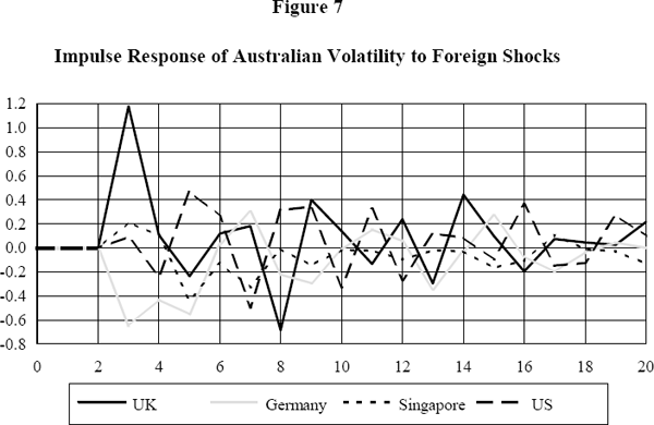
The impulse response functions come from inversion of a VAR model, via the Wald transformation, to a moving-average representation. The advantage of the impulse-response function is that it allows ‘innovation accounting’. In this procedure, one sets all initial values to zero, and shocks one of the variables to a unit value at time t = 1. The response function indicates what happens to the system in succeeding periods, from period t = 2 onwards, if no further shocks occur. In Figure 7, the impulse response extends twenty periods[6].
Figure 7 shows that the largest response comes from a unit shock in the UK volatility measure. A one percent increase in volatility of the Financial Times index leads, within three months, to a 1.2 percent increase in volatility in the Australian index. An increase in volatility in the German market actually dampens volatility in the Australian index for the first five months. Figure 7 also shows that the effects of the external volatility shocks have their largest effects within six months[7].
Further information about the relative importance of domestic and foreign shocks for the Australian stock price volatility is given by examining the proportion of the variance of the forecast error at differing horizons, which are due to each of the shocks. These variance decompositions appear in Table II[8].
| Horizon | Percentage of Variance Due To: | |||||
|---|---|---|---|---|---|---|
| Australia | Germany | Japan | Singapore | UK | US | |
| 1 | 46.27 | 0 | 3.15 | 1.59 | 48.70 | 0.29 |
| 5 | 36.99 | 0 | 17.53 | 5.73 | 31.95 | 7.80 |
| 10 | 25.42 | 0.96 | 26.12 | 5.18 | 28.61 | 13.71 |
| 15 | 23.91 | 1.20 | 24.76 | 5.17 | 30.01 | 14.94 |
| 20 | 23.01 | 1.63 | 24.99 | 5.26 | 29.43 | 15.67 |
| 40 | 22.63 | 1.70 | 24.99 | 5.37 | 29.39 | 15.92 |
| 60 | 22.61 | 1.70 | 25.00 | 5.37 | 29.38 | 15.93 |
Table II shows clearly that forecast errors of the Australian rate at both short and longer horizons are about equally due to shocks in the UK Financial Times index as to the Australian rate itself. The Nikkei index becomes more important at longer intervals, even more important than the Australian rate at 40 and 60 month horizons. Thus, variance-decomposition analysis reveals a more important role for volatility in the Nikkei index than does analysis of contemporaneous correlations or the impulse-response function.
2.4. Analysis of Time-Varying Return Coefficients
The time-varying return coefficients for the Australian stock index are obtained from Kalman-filter estimation of the following model:
where [ΔsG,t ΔsJ,t ΔsS,t ΔsUK,t ΔsUS,t] is the matrix of logarithmic first differences of the German (G), Japanese (J), Singapore (S), British (UK) and Dow-Jones (US) stock indices at time t, ΔsA,t is the first difference of the Australian return at time t, [βt δt] are the time-varying coefficient matrices of the contemporaneous foreign returns and lagged own return, and εt is a random variable, with independent and identical distribution.
Kalman-filter estimation of the coefficients in equation (1) allows us to see how returns across countries become more closely linked during periods of high or rising volatility. In this sense, the time-varying parameters in (1) represent ‘contagion’ coefficients, which should be closely correlated with the volatility measures[9].
The Kalman filter method is described in Hansen and Sargent (1991). Equation (1) is estimated in a recursive manner, in which the coefficients evolve so as to give the best one-period forward predictions. The updating of the coefficients is based on an error-correction or learning mechanism, in which current and more recent forecast errors weigh more heavily than past forecast errors for updating the coefficients. Unlike rolling regressions, Kalman filtering allows an optimal discounting of past data, so that the more recent observations and forecast errors have more influence on the parameter values. With rolling regressions, all observations have equal weight[10].
Figure 8 pictures the paths of the coefficient of the UK stock return and the Australian lagged return during the sample period.
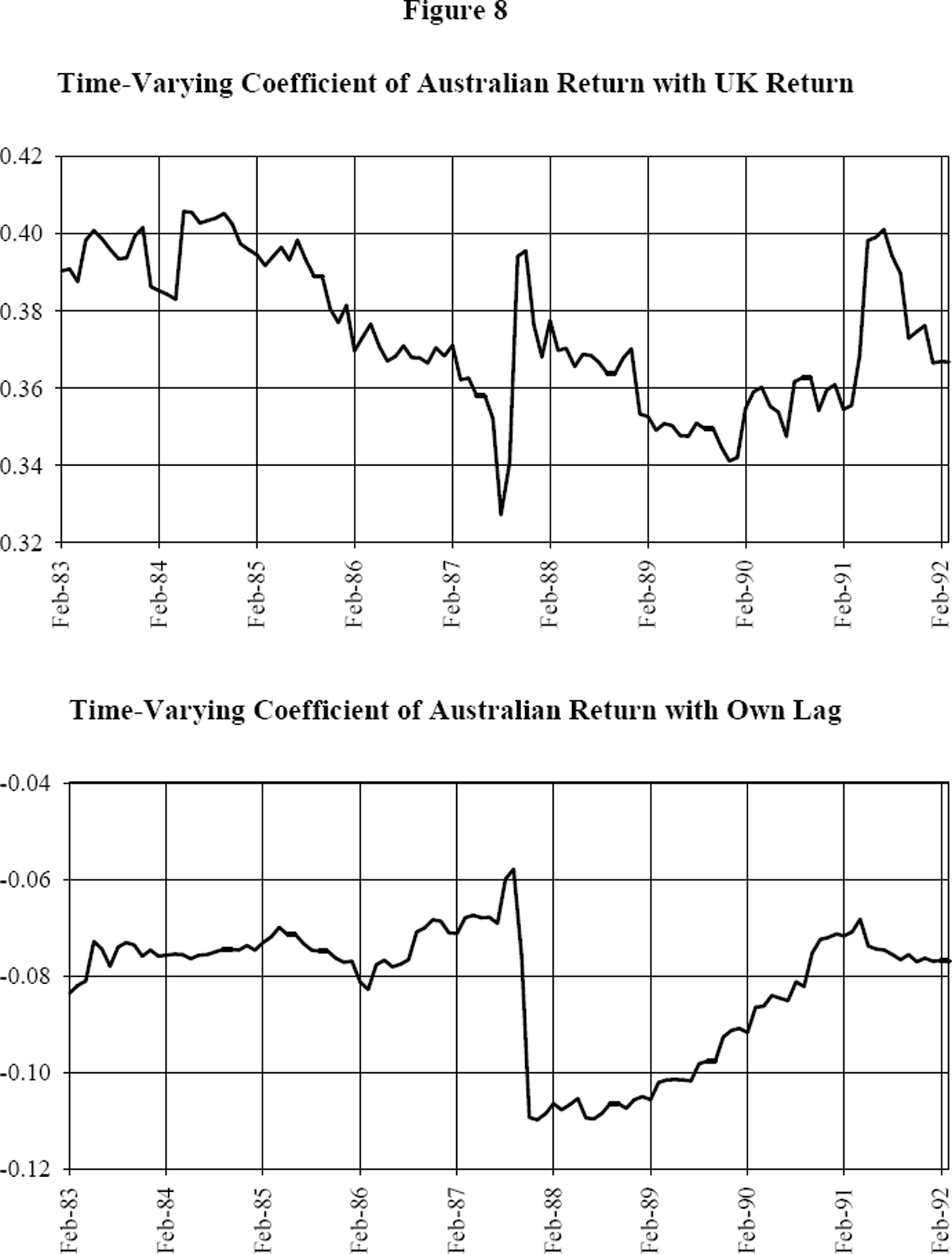
Both time-varying estimates show sharp jumps at the time of the 1987 crash. Before the crash, the correlation of the Australian return with the UK return was gradually diminishing, but it increased by about 20% on the crash date. Figure 8 also shows that there was a large increase in the negative serial correlation of the Australian index on ‘Black Tuesday’.
Table III contains the correlations of the two time-varying return coefficients with the international volatility measures, during the turbulent period from 1987.01 through 1988.12[11]. This sub-sample is chosen, because it is the period prior to and following ‘Black Monday’, when stock-market turbulence was highest. The correlations show that, during the two year period, volatility in the UK and US markets increased in tandem with the return coefficient linking the Australian rate to the UK rate. Given the negative sign of the time-varying Australian autocorrelation coefficient, the positive correlations indicate that as volatility increased in all of the markets, the Australian autocorrelation coefficient diminished in absolute value. The market became progressively more responsive to international prices as international turbulence grew, and less dependent upon its own history.
| Volatility Index: | Coefficients | |
|---|---|---|
| βUK,t | δt | |
| Australia | 0.2643 | 0.2395 |
| Germany | 0.3337 | 0.1272 |
| Japan | 0.2405 | 0.1794 |
| Singapore | 0.1915 | 0.1454 |
| UK | 0.3069 | 0.2723 |
| US | 0.5068 | 0.1263 |
Footnotes
In several cases, the Schwert volatility measures become negative. This is a drawback of this measure. Pagan and Schwert (1989) point out the importance of non-linearities in stock return behavior that can be captured neither by the ARCH nor GARCH model, nor by the Schwert measure, of asset-price volatility. [4]
See Judge, Hill, Griffiths, Lutkepohl, and Lee (1988) for a description of the Wald statistic for testing linear restrictions. [5]
See Judge, Hill, Griffiths, Lutkepohl, and Lee (1988), pp. 771–776, for further information on this method. In the MATLAB program, the initial period is t=1, so that the initial shock occurs at t=2 and the responses appear by t=3. [6]
While the stock market volatility in several foreign markets causes a decline in Australian volatility, the only significant volatility effect, from the UK, is strongly positive for the initial periods. [7]
See Lowe (1992) for an application of variance-decomposition analysis to Australian real exchange rates. [8]
By the simple efficient markets theory, under the assumption of risk neutrality, the logarithmic stock price index should behave as a random walk. Thus, [δt] should not depart from zero, since the vector is a set of coefficients of data observed at time t−1. Any increase in the absolute values of the coefficients in this matrix when volatility measures are higher than normal indicates a departure from market efficiency, narrowly defined. The contagion model permits such a departure, even for ‘efficient markets’. Thus, my use of time-varying parameter estimation during times of increasing volatility is not an ‘excess-volatility’ test of market efficiency. Shiller's (1989) ‘excess volatility’ tests are based solely on present-value models of asset price behavior and rational expectations and do not consider international linkages of volatilities. [9]
Unfortunately, the distribution of the Kalman filter coefficients is not known so it is not possible to test if movements of the time-varying coefficients beyond specified bounds indicate significant departures from particular parameter values. [10]
Only two coefficients appear in Table III, that of Australia with the UK stock index, and the Australian index with its own lag, because these are the only coefficients which showed significant variation in the Kalman filter estimation. Table III shows the correlations of these Kalman coefficients with the volatility indices for the five countries to show the different ways these time-varying parameters are related to uncertainty measures in the various markets. [11]
