RDP 9208: Credit Supply and Demand and the Australian Economy Appendix A: Maximum – Likelihood Estimation of the Demand and Supply of Business Credit

1. The Likelihood Function

The model that we estimate is:

where D_t denotes the quantity demanded during period t, S_t the quantity supplied during period t, χ_Dt and χ_St denote the exogenous variables that influence D_t and S_t respectively, and u_Dt and u_St are the residuals. It is assumed that the observed quantity of loans transacted is the minimum of demand and supply. That is, as in any market with voluntary exchange, the short side of the market must prevail. Thus, let Q_t be the actual quantity observed during period t:

Maddala and Nelson (1974) derive the likelihood function for this model using limited – dependent variable methods.

The probability that the observation Q_t belongs to the demand equation is given by:

It is assumed that uD and uS are independently and normally distributed, with variances and respectively (and that they are also serially independent). Therefore, u_D − u_S is normally distributed with variance σ² = + .

Hence,

Now define,

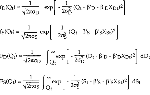
Then, given that Q_t belongs to the demand equation, the conditional density of Q_t is given by:

The denominator of this is equal to pr(D_t < S_t) and, hence, is equal to π_t. Thus this can be written as:

Similarly, the conditional density of Q_t, given that Q_t belongs to the supply equation, is written as:

Since Q_t lies on the demand equation with probability π_t and on the supply equation with probability (1 − π_t), the unconditional density of Q_t (given the observed values of the exogenous variables χ_Dt, χ_St) is as follows:

Hence, the log – likelihood, L, may be written as:

where n is the number of observations.

2. The Estimation Method: Discussion

Parameter estimates were obtained by maximising the log – likelihood using the Broydon, Fletcher, Goldfarb and Shanno (BFGS) maximisation algorithm (which is a modification of the Davidon, Fletcher, Powell method).

A number of caveats are in order when estimating models with unknown sample separation. Firstly, a conceptual problem arises in that too much may be asked of the data when it is not known which observations are on the demand function and which are on the supply function. Monte Carlo methods find that there is considerable loss of information if sample separation is not known. However, empirical results obtained by some other studies using this method are quite good (Maddala (1983) p 299).

Secondly, it can be shown that the likelihood function for this model is unbounded for certain parameter values. However, it has been shown that even if the likelihood function diverges, a consistent estimate of the true parameter value in this model corresponds to a local maximum of the likelihood function, rather than a global maximum. Thus the fact that a local maximum is obtained rather than a global maximum is not a matter of concern, but this result does not ensure that the particular local maximum we have located will give a consistent estimate of the true parameter values.

Finally, the estimate of the covariance matrix produced by the BFGS method may not be precise. The estimated covariance matrix from the BFGS algorithm is (for a well – behaved function) approximately -H, where H is the Hessian of the objective function L. The only exact result that holds for the BFGS method is that if L is quadratic with K free parameters, then after K or more iterations the estimated covariance matrix will be exactly -H (Doan (1988). However, the log-likelihood from our model is considerably more complex than a quadratic function, hence standard errors reported in this paper should be interpreted as a guide to significance, rather than as a precise measure of significance.