RDP 9102: Indicators of Economic Activity: A Review 4. Partial Indicators
March 1991
- Download the Paper 384KB
This section looks at the performance of partial indicators in four main areas: housing, investment, consumption and the labour market. The usefulness of these indicators arises potentially from two sources. First, they are often published as monthly series and have considerably shorter publication lags than the national accounts. This provides an important, purely mechanical, reason why such indicators can provide useful information. Secondly, it is possible that they lead the broader spending and production aggregates in terms of underlying timing, and it is this possibility that is examined in the empirical tests reported below.
(a) Housing
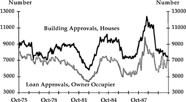
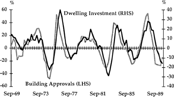
The formalities involved in the process of constructing dwellings provide a well-defined set of potential leading indicators for investment in the housing sector. Securing a housing loan commitment by owner-occupiers is one of the first identifiable links in the chain. Subsequently, a building approval is needed from the relevant local authority before work can commence. Data on new loan approvals and building approvals are published by the ABS with a lag of one to two months, with the building approvals data generally being the earlier of the two to be published. The national accounts measure of dwelling investment is the value of work done, which can diverge from building approvals for essentially two reasons: first, a small proportion of approved dwellings are not commenced, and secondly, roughly half the value of work done is on alterations and additions, which are not covered in the approvals data. These points aside, one would expect building approvals to lead work done, due simply to the average time required for completion. These relationships are illustrated in Graphs 7 and 8.
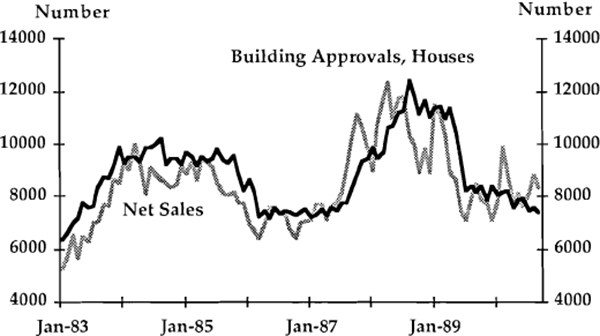
A further indicator of house building approvals is provided by the Housing Industry Association's survey of volume builders. The HIA defines net sales of new houses as the number of deposits taken by volume builders for the drawing up of plans, less cancellations. As Graph 9 indicates, the historical net sales series appears to have a leading relationship to building approvals; however, it should be noted that it is a fairly volatile series and it is also prone to frequent revisions, both of which diminish its value as a forward indicator.
The estimated forecasting equations reported in Tables 7 and 8 provide strong support for the observations made above. In bivariate systems (Models 1 and 2 in Table 7) both building approvals and housing finance have statistically significant power to forecast dwelling investment when the other variable is excluded. The relationship appears strongest in the case of building approvals, which forecasts investment with an R-squared of 0.59. The most significant lags appear to be the first and second, suggesting an average lead time of three to six months for this indicator. Interestingly, the contemporaneous value of building approvals adds little to the explanatory power of the equation, raising the R-squared only from 0.59 to 0.62. When the system as a whole is estimated (Model 3), the result is obtained that only the building approvals series enters as a significant predictor of dwelling investment; housing finance does not add significantly to the information in the building approvals series.
| Model 1 | Dwelling Investment |
Approvals | |
|---|---|---|---|
| Dwelling Investment | 0.6 | 18.6* | |
| Approvals | 1.5 | 7.5* | |
| Model 2 | Dwelling Investment |
Finance | |
| Dwelling Investment | 1.7 | 6.2* | |
| Finance | 1.8 | 1.7 | |
| Model 3 | Dwelling Investment |
Approvals | Finance |
| Dwelling Investment | 3.3* | 7.8* | 1.3 |
| Approvals | 0.8 | 1.6 | 0.5 |
| Finance | 0.6 | 1.0 | 0.6 |
|
Note: All equations are estimated over the period 1969(4) to 1989(2), (79 observations) with three lags. The table shows F-statistics for the test of the null hypothesis that the lag coefficients on a variable are jointly zero. Asterisks denote significance at the 5 per cent level. |
|||
| HIA | Finance | Approvals | |
|---|---|---|---|
| HIA Net Sales | 1.2 | 1.1 | 0.4 |
| Finance | 3.8* | 5.1* | 1.2 |
| Approvals | 2.6* | 0.8 | 6.7* |
Note: The system is estimated using monthly data over the period 1983(8) to 1986(6), (71 observations), with six lags. Otherwise, notation conforms to that in previous tables. |
|||
The above quarterly regressions were implemented by aggregating the relevant monthly numbers to obtain quarterly totals for the two partial indicators which were then used in predicting the quarterly national accounting aggregate. Because this procedure throws away some information from the monthly series, it is of interest to look further at the inter-relationships between the monthly indicators. This also allows sufficient observations to bring in the HIA series, which is only available from 1983. The results for a three-variable VAR using monthly data on sales, finance and approvals are summarised in Table 8. The net sales series is found to contain statistically significant leading information on both finance and building approvals, with the profile of coefficients suggesting that lags of up to about four months are significant. Unfortunately, the short data series prevents direct testing of the link from sales to the national accounts aggregate of work done, but the results seem to provide robust support for two conclusions: that building approvals form a reliable leading indicator of work done, and that net sales lead approvals. Housing finance is also a leading indicator of work done but cannot statistically be shown to add to the information contained in the other two variables.
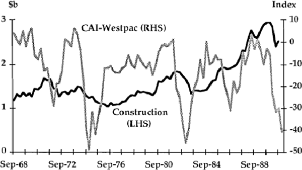
(b) Business Investment
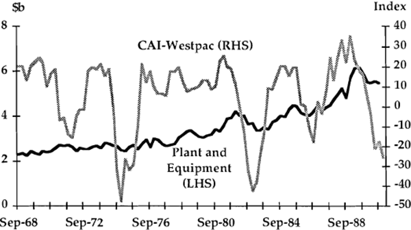
The main partial indicators of business investment are provided by two surveys of investment intentions, the ABS Capital Expenditure survey (CAPEX) and the CAI-Westpac survey of the manufacturing sector: each survey is conducted quarterly. In the ABS survey, respondents are asked to report their investment intentions in value terms, allowing their responses to be aggregated to obtain an estimate of the total. Generally this has been found to result in underestimates of investment, and for forecasting purposes the figures are usually adjusted to compensate for this. The CAI-Westpac survey follows the somewhat simpler procedure of asking businesses whether they expect their investment levels in the coming year to rise, fall or stay the same. An index of investment intentions is then obtained by taking the difference between the proportion of respondents expecting a rise, and the proportion expecting a fall. This difference is referred to as the net balance (see Graphs 10 and 11).
Two features of the ABS survey make it difficult to translate the numbers directly into quarterly forecasts. The first is the structure of the reporting cycle, whereby expectations are reported only as half-year and annual totals; this means that in two quarters out of four a direct quarterly forecast can be inferred by deducting the relevant quarterly outcome from the half-year forecast, while in the other two cases only the half-year figure is available. Moreover, these figures are not adjusted for under-reporting bias or seasonal factors. Secondly, the CAPEX expectations are forecasts of CAPEX outcomes, rather than national accounts outcomes, for business investment. This second problem is relatively minor in the case of equipment investment, where the two series are similar, but is quite serious for construction, as will be discussed further below.
In view of the complications referred to above, the forecasting equations to be estimated are set up as follows. First, business investment is divided between its equipment and construction components. For each component, quarterly CAPEX forecasts are constructed for the quarters where direct forecasts are not available, by simply halving the half-year forecasts. Forecasting equations are then set up, using the relevant survey variables to predict investment outcomes. In the case of construction investment, a series on non-residential building approvals is also included. The equations are estimated in non-seasonally-adjusted nominal terms, since that is the form in which the forecasts are expressed; seasonal dummies are included to allow for possible seasonality in the prediction errors. Results for the two sets of forecasting equations are presented in Tables 9 and 10.
| Independent Variable | ||
|---|---|---|
| CAI/Westpac (Lags 1 to 4) |
CAPEX Forecast (Lag 1) |
CAPEX Forecast (Lags 1 to 4) |
| 1.13 | ||
| 1.76 | 2.80* | |
| 17.36* | ||
Note: The table shows F-statistics for the null hypothesis that the relevant coefficients are zero. The data period is 1975(2) to 1988(4), (55 observations). The dependent variable in each case is the nominal quarterly growth of plant and equipment investment (national accounts basis, n.s.a.). All equations include four lags of the dependent variable and seasonal dummies. |
||
| Independent Variables | ||||
|---|---|---|---|---|
| Dependent Variable | CAI/Westpac (Lags 1 to 4) |
Construction Approvals (Lags 1 to 4) |
CAPEX Forecast (Lag 1) |
CAPEX Forecast (Lags 1 to 4) |
| Construction (National Accounts basis, s.a.) |
2.76* | |||
| Construction (National Accounts basis, n.s.a.) |
2.90* | |||
| 4.20* | ||||
| 0.60 | 1.61 | |||
| 1.83 | ||||
| Construction (CAPEX basis, n.s.a.) |
32.86* | |||
| 10.53* | ||||
Note: All equations include four lags of the dependent variable. Seasonal dummies are included in all equations except the first. Data are not seasonally adjusted except for the dependent variable in equation 1. The data period is 1975(2) to 1989(2), (55 observations). Asterisks denote significance at the 5 per cent level. |
||||
For plant and equipment investment (Table 9), the results indicate that CAPEX forecasts are significant predictors of investment, but that the CAI-Westpac index does not contain significant additional information. Indeed, if all information other than the first lag on the CAPEX forecast is excluded, the forecasting equation still has an R-squared as high as 0.92 (although it should be noted that much of the explanatory power is contributed by the seasonal dummies). In the case of construction however (Table 10) both the CAPEX and CAI-Westpac forecasts performed poorly. Building approvals do appear significant, with a peak lag coefficient coming at three quarters, suggesting quite long average implementation lags in construction projects. It would appear that the poor performance of the CAPEX construction forecast is due largely to the lack of correlation between the national accounting and CAPEX estimates of actual investment outcomes. In other words, the CAPEX forecasts are useful for predicting CAPEX outcomes, but not national accounting outcomes.[4] This is evident from the last equation reported in Table 10, which shows that when the dependent variable is the CAPEX measure of construction investment, rather than the national accounts measure, the forecasts are highly significant.
This last qualification aside, the above results suggest that good forward indicators are available for both major components of investment spending. The study has not addressed the accuracy of the longer-range forecasts (out to seven quarters ahead) which are also reported in the CAPEX surveys. However, a recent study by Brennan and Milavec (1988) suggested that these longer-range forecasts are much less accurate, and that their prediction errors could not be accounted for by unexpected developments in other economic variables. Taken in conjunction with the results reported here, this would imply that the main usefulness of the CAPEX forecasts is in short-term forecasting, particularly the next quarter ahead.
(c) Consumption
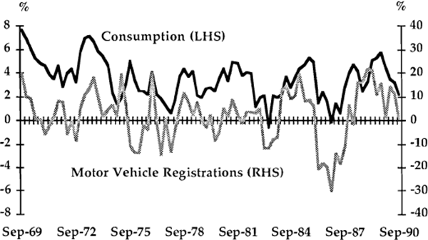
Three main partial indicators of consumption are in common use; retail trade, motor vehicle registrations and the index of consumer sentiment: all are published monthly. The first two are components of aggregate consumption spending, comprising about 40 per cent and 4 per cent of the total respectively. Being such a large proportion of the total, retail trade data convey important information for the purely mechanical reason that they are available with shorter publication lags than the national accounts (about two months). Unfortunately, however, the interpretation of these figures is hampered by the presence of considerable month-to-month variation, which is especially evident during the past four years. This is mainly a consequence of problems in seasonal adjustment, caused for example by frequent changes to the timing of school holidays, which have had a significant effect on the seasonal pattern of consumer spending. Motor vehicle registrations are considered a useful indicator because of their relatively short publication lags, and because this is probably, together with household durables, one of the principal areas of consumption which is sensitive to policy change (see Graph 12).
The Melbourne Institute's Index of consumer sentiment reports results of a consumer attitude survey containing five questions on a variety of topics, including the respondent's present and expected financial position, and the suitability of the present time for major household purchases. The index is constructed from balances of favourable over unfavourable responses averaged over the five questions.
Estimates from the forecasting equations using the three indicators are reported in Table 11. These suggest fairly unambiguously that motor vehicle registrations contain significant leading information about aggregate consumption. Estimates of individual lag coefficients show the strongest effect occurring at a lag length of two quarters. Neither retail trade nor the consumer sentiment index is found to add significantly to predictive power. These results should not however be taken as detracting from the usefulness of the retail trade data in the mechanical sense referred to above.
| Con. | RT | CS | MVR | |
|---|---|---|---|---|
| Consumption | 2.7* | 0.7 | 0.9 | 3.2* |
| Retail Trade | 2.8* | 0.9 | 0.1 | 3.2* |
| Consumer Sentiment | 1.4 | 0.6 | 0.7 | 0.4 |
| Motor Vehicle Registrations | 0.9 | 1.2 | 2.5 | 0.7 |
Note: Notation and data period are as in Table 7. |
||||
(d) Labour Market
Monthly labour market indicators of employment and job vacancies are among the most quickly published indicators of the real economy. Publication lags are usually less than two weeks, compared with six to eight week delays for retail sales and the monthly housing indicators. Employment data are obtained from the ABS labour force survey, while monthly job vacancies figures are provided by the ANZ bank from a survey of job advertisements in major newspapers.[5] Comparisons between employment and GDP, vacancies and employment, and vacancies and GDP, are shown in Graphs 13, 14 and 15 respectively.
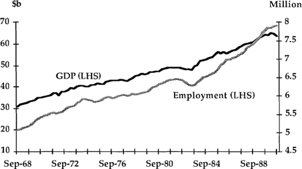
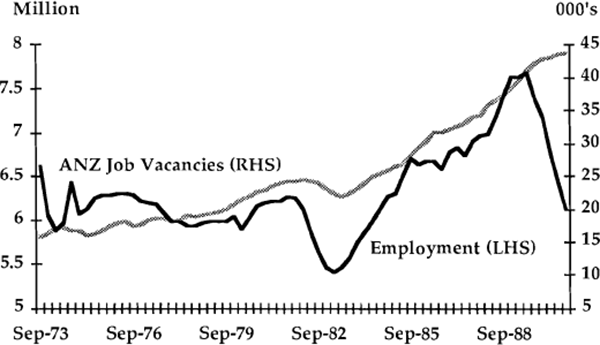
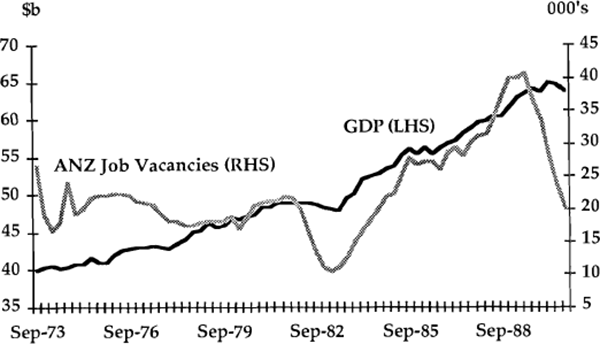
Major slowings in employment growth occurred in 1974 and 1982 (Graph 13). In the former case, the slowing clearly preceded a slowing in GDP growth, whereas in 1981, employment moved together with, or slightly behind, output. The difference between the two cases can probably be attributed, at least in part, to the differing behaviour of real wages in the two cycles. In the 1974 episode, major real wage increases occurred much earlier, relative to the cycle in GDP, than was the case in 1981. The milder slowing in employment growth which occurred in the second half of 1986 provides a further perspective on the issue. With real wages remaining fairly constant through the cycle, the slowing in employment growth followed that of real GDP by two or three quarters. The ANZ job vacancies series appears to have acted as a reasonably good forward indicator of trends in employment (Graph 14). Job vacancies led the downturn in employment growth in both 1981 and 1986.
Estimated forecasting equations summarised in Table 12 suggest that the ANZ vacancies series is a significant predictor of both GDP and employment. In the GDP equations the first quarterly lag is highly significant, a result which seems fairly robust to changes in the number of lags included. The employment equation is estimated using monthly data and shows the vacancies coefficients to be jointly significant when up to nine lags are included, with the highest coefficient occurring at a lag of three months.
| Dependent Variable |
Data Frequency |
Number of lags |
Independent Variables | |
|---|---|---|---|---|
| Vacancies | Employment | |||
| GDP | quarterly | 4 | 4.75* | 0.53 |
| 3 | 4.90* | 1.28 | ||
| 2 | 5.12* | 0.03 | ||
| 2 | 5.47* | |||
| 1 | 9.03* | |||
| Employment | monthly | 9 | 2.51* | |
| 6 | 2.85* | |||
Note: All equations are estimates with lagged dependent variables. Data periods are 1974(1) to 1989(2) for quarterly equations, and 1978(9) to 1989(6) for monthly equations. Asterisks denote significance at the 5 per cent level. |
||||
Footnotes
The two series differ partly for reasons of coverage, and partly because the CAPEX survey records investment spending, whereas the national accounts series are a measure of the value of work done. [4]
A quarterly survey of job vacancies is also published by the ABS, but is not studied here. [5]