RDP 9001: Is Pitchford Right? Current Account Adjustment, Exchange Rate Dynamics and Macroeconomic Policy 2. The Market-Clearing Model

Models which incorporate the dynamic interaction between the price of foreign assets (the exchange rate) and the rate of accumulation of those assets (the current account) date back to Kouri (1976).^[4] These models integrate the notion that the exchange rate is an asset price with the insight that changes in net asset holdings can only come about through current account imbalances. They also highlight the intertemporal nature of the relationship between the current and capital accounts, and the effects of this connection on exchange rate determination.

The model in this paper draws heavily on Mussa (1984). The model consists of a home country which trades two goods (domestically produced goods and foreign goods) with a foreign country. Also traded is a real asset, which pays a fixed rate of return in terms of foreign goods equal to r, the foreign real interest rate. The stock of this asset held by domestic residents, denoted a, may be positive or negative.

Foreign residents are willing to exchange foreign goods for real assets at the prevailing rate of return r; however, their demand for domestic goods in exchange for foreign goods is less than perfectly elastic with respect to the relative price of those goods (the real exchange rate). Consider equations (1) – (3).

d is the value of domestic excess demand for domestic goods, d^* is foreign excess demand for domestic goods (the home country's real exports), f is domestic excess demand for foreign goods (the home country's real imports) and ψ is the excess of domestic spending over the value of domestic product. All of the above are measured in units of the foreign good. σ is the marginal share of domestic goods in domestic spending. q is the logarithm of the price of domestic goods in terms of foreign goods, so an increase in q represents an appreciation of the home country's real exchange rate. β and β^* are semi-elasticities. x, y and z are exogenous shocks to d, d^* and f respectively. Note that equations (1) and (3) are constrained so that d + f = ψ.

Equilibrium in the market for domestic goods occurs when

Assume, for simplicity, that β + β^* = 1.^[5] From (4), we can then derive

where v = 1/σ.

By definition, the real trade surplus T = d^* − f. It is easy to show that T = −ψ i.e. T is equal (as it should be) to the excess of domestic production over domestic spending.

From (5), we can see that an increase in q (a real appreciation) reduces the trade surplus, as does an exogenous increase in imports, z. An increase in x, the exogenous component of domestic spending on domestic goods, appears to increase the trade surplus. However, this is not the case. An increase in x must be offset by decreased demand for domestic goods to maintain equilibrium in that market. This occurs via an appreciation of the real exchange rate, which leads to a decrease in real exports and an increase in real imports, hence leading to a trade deficit.

Finally, it appears that an exogenous increase in the foreign excess demand for domestic goods, y, leads to an improvement in the trade balance, but this is also not the case. The apparent effects of the increase in y are eliminated by an increase in q, which results in offsetting changes in imports and exports. There is no effect on the trade balance. The intuition behind this result lies in the fact that the trade balance identically equals the difference between domestic savings and investment. Changes in foreign spending propensities, as given by y, have no effect on domestic savings or investment behaviour, and so must therefore have no effect on the balance of trade.^[6],^[7]

The current account balance in year t is given by the sum of the trade balance and the foreign income account:

(The values of x, y, and z are assumed to be constant and so the time subscript on these variables is suppressed).

As a matter of accounting, the accumulation of net foreign assets by domestic residents in year t is equal to the current account balance in year t.^[8] Thus,

where a_t denotes net foreign assets held at the beginning of t. In equilibrium, savings is equal to desired savings. The latter is assumed to be given by

where R_t is the domestic real interest rate, A is a target level of foreign assets, and u is a parameter. Desired savings in period t is a fraction u of the difference between the targeted and realized level of foreign assets, and an increasing function of the real interest differential between the home and foreign country.^[9] Exogenous domestic spending on domestic and foreign goods is assumed to reduce desired savings one for one.

R_t is determined by the interest parity condition

where E_t(q_t+1 − q_t) is the expected appreciation of the real exchange rate between periods t and t+1. According to equation (9) an asset that yields a rate of return r_t in terms of foreign goods will yield a rate of return in terms of a domestic consumption basket equal to r_t less the expected rate of increase of the relative price of domestic goods, weighted by the share of domestic goods in the consumption basket.

The expected change in the real exchange rate is determined by

where is the steady state value of q. Equation (10) says that the expectation, held at time t, of the change in the real exchange rate between t and t+1 is equal to a proportion of the difference between its steady state value and its realized value at t. As savings become more responsive to a discrepancy between realized and targeted assets (an increase in u), the faster will the real exchange rate be expected to converge to its steady state value.

Substituting (9) and (10) into (8), and equating with (6), yields

From equation (11), we can see that an increase in the target level of real foreign assets, A, leads to a depreciation of the real exchange rate. This occurs because larger trade surpluses are needed in order to accumulate these assets. An increase in the actual level of such assets, on the other hand, leads to a real appreciation. An increase in the foreign interest rate, r, results in a depreciation if the level of foreign assets is negative, since larger trade surpluses are needed to meet the new, higher, interest payments on the debt. The converse occurs if the country is a net creditor.

The exogenous component of domestic spending on domestic goods, x, affects q directly and indirectly through its effects on a. On the other hand, y, exogenous foreign spending on domestic goods, has no such indirect effect, since it doesn't affect the current account balance. Finally, z, the exogenous component of real imports, has no direct effect on q, but it has an indirect effect through a.

Equations (7) and (11) jointly determine the time paths of the stock of real foreign assets, a, and the real exchange rate q. The steady state is reached when asset accumulation (or decumulation) is zero, i.e. the current account balance is zero. In the steady state the trade balance exactly offsets the interest receipts (or payments) on the stock of net foreign assets. A bit of algebra reveals that the steady state values of a, q and T (respectively â, and , are given by:

x, y and z can be thought of as permanent spending shocks, each with an initial value of zero. From (12), we can see that permanent increases in x and z lead to a permanent fall in the steady state value of domestically held foreign assets. The extent of the fall varies inversely with u, the savings adjustment parameter. The more sensitive are savings to shortfalls in the level of foreign assets, the smaller will be the eventual decline in foreign asset holdings following (positive) shocks to domestic spending. (Of course, there will be no fall in the steady state value of a if these shocks are temporary.)

From (12), it is clear that permanent increases in y have no permanent effects on a, in fact, they don't even have temporary effects. Substitution of (13) into (11) reveals that following a change in y the real exchange rate immediately jumps to its steady state value, with asset accumulation unaffected.

Abstracting from the effects of exogenous spending, we can see from (13) that if A is positive (negative), q takes on a positive (negative) value in the steady state. From equation (14), a positive (negative) value of A implies that income from foreign assets is positive (negative); this must be offset by a trade deficit (surplus) to yield a zero current account balance.

From (13), a permanent increase in exogenous real imports unambiguously depreciates the real exchange rate in the long run. It is interesting to note, however, that x shocks have an ambiguous effect on the steady state value of the real exchange rate.^[10] While the impact effect of positive x will be to increase q, q will be smaller (than its initial value) in the steady state if the following condition holds:

The intuition behind this result is that, on the one hand, following a positive x shock, the real exchange rate needs to appreciate to maintain equilibrium in the market for domestic goods. On the other hand, the initial current account deficits lead to an accumulation of foreign debt; trade surpluses are needed to cover the interest on this debt, and the real exchange rate will need to depreciate to generate these surpluses. These effects tend to offset each other, with the final outcome depending on the parameter values.

If u is relatively small, savings will adjust slowly to the initial debt and the final build-up in debt will be relatively large. This implies a large incomes deficit on the current account, and so, on balance, the real exchange rate will depreciate relative to its initial value.

The stability condition for this model is easily determined. For non-zero u, it is

This is an extremely weak condition. A plausible value of v is about 1.7, (assuming that σ is about equal to 0.6). This implies that r need only be less than 2.8 for the model to be stable i.e. for the level of debt to reach a permanent maximum. Since one very rarely observes annual real interest rates of around 280 per cent, it seems safe to conclude that unsustainable debt traps are extremely unlikely to occur.

However, if u = 0, the model is unstable at any real interest rate, and the level of debt does indeed become infinite. This is what most commentators have in mind when asserting the existence of a debt trap. With a trade balance of zero, the level of debt must go to infinity, as a matter of arithmetic, if the real interest rate on that debt exceeds the real growth rate of output. Since output in this model does not grow, any positive real interest rate will yield an infinite amount of debt, provided that u = 0.

The problem with this scenario is that u = 0 implies that economic agents make absolutely no adjustments to their spending and savings patterns when confronted with debt. In other words, it implies that people and firms will voluntarily send themselves into bankruptcy. As a theory of economic behaviour for individuals, this reasoning is, at best, dubious; applied to the nation as a whole, it becomes preposterous. One can only conclude that popular commentators who assert the existence of an unsustainable debt trap need, at the very least, to explain more precisely how such a predicament can arise.

Some Illustrative Simulations

For simulation purposes, values have to be assigned to five parameters: A, r, u, β and σ. Without loss of generality, A can be set at zero; r is assumed equal to 0.05; u is assumed to be equal to 0.25; β is set at 0.5 and σ is set at 0.6.^[11] Figures 1 to 8 illustrate the effects of a 0.20 permanent upward shock to x and z on the trade and current account balances, level of debt, real exchange rates, imports and exports. The initial values of all the variables is zero, and the shocks occur in year zero. Consider the shock to x, exogenous domestic spending on domestic goods.

REAL DOMESTIC EXPENDITURE SHOCK (x)

REAL IMPORT SHOCK (z)

u = 0.25

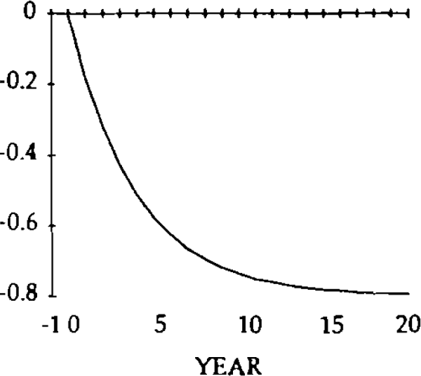
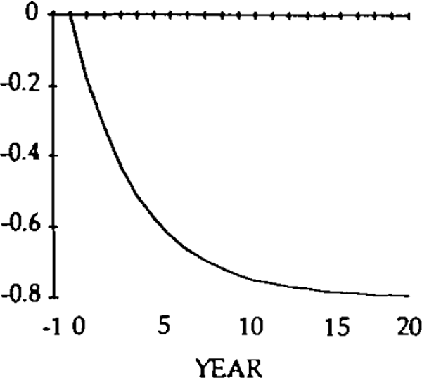
Figure 1 shows the effect on net foreign assets. Following the initial trade deficit, debt accumulates for about fifteen years, before reaching its steady state value of x/u. The time taken to reach this steady state depends crucially on the value of the parameter u. If u were larger, indicating that desired savings were more responsive to discrepancies between targeted and realized net foreign assets, then the level of debt would stabilize much more quickly, and at a lower level. For example, if u = 0.75, the steady state would be reached in about five years, and with debt one-third the level shown in figure 1.

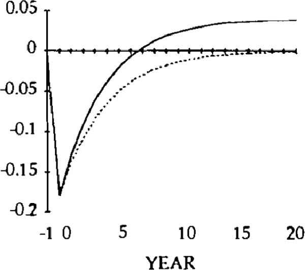
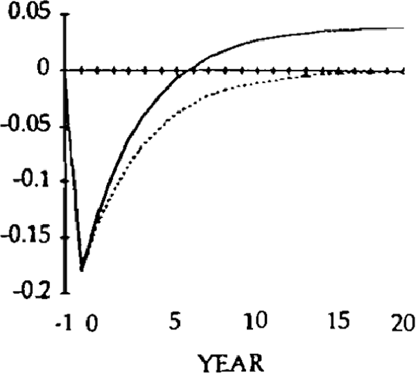
Figure 2 shows the effects of the shock on the trade balance and the current account. Following the spending shock, both the trade balance and current account are in a deficit position. Over time, this deficit gradually becomes smaller. The trade balance becomes positive after seven years, but, because of the interest payments on the debt, the current account is still in a deficit position. A further eight years of trade surpluses are required before the current account becomes balanced.

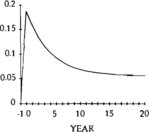
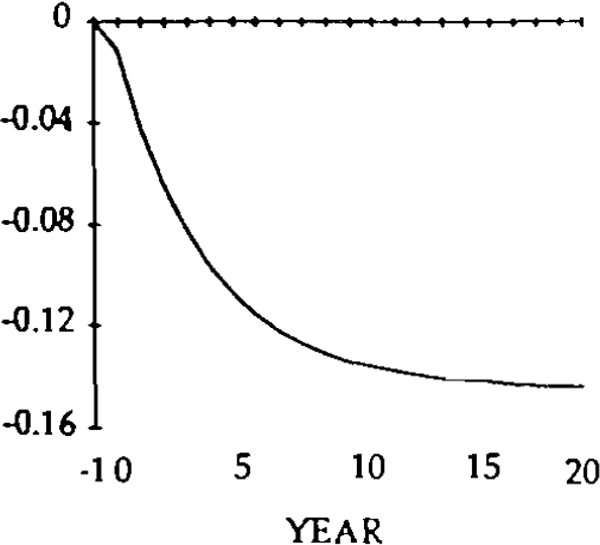
Figure 3 plots the effects on the real exchange rate. After an initial jump, it gradually falls back to its steady state value.

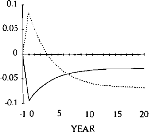
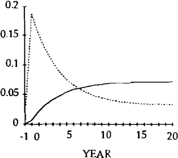
Figure 4 displays the paths of exports and imports. The initial real appreciation leads to a fall in exports and a rise in imports. In the new steady state, exports have fallen somewhat below their initial value of zero, and imports have fallen considerably below this level. This large fall in imports is necessary to create the trade surplus necessary to maintain a balanced current account, given the steady state level of foreign debt.

Figures 5–8 show the effects of a z shock.

A comparison of figures 2 and 6 shows that the dynamic paths of the trade balance and current account are identical under each type of domestic spending shock; thus, so are the paths for debt. This is as expected since the x and z shocks reflect identical reductions in desired savings. However, the paths for exports and imports and the real exchange rate are different.

A z shock leads to an initial jump in imports, which gradually falls (as the real exchange rate depreciates) but is still positive in the new steady state. Exports, on the other hand, gradually rise throughout the adjustment process. Thus, under the two kinds of spending shocks, the difference between exports and imports – the trade balance – is identical in every period, but the components of the trade balance follow very different adjustment processes. These differences can be traced to a different adjustment path for the real exchange rate.

The results of this section show that, even following permanent adverse shocks, a current account deficit will, eventually, correct itself, and the level of foreign debt will stabilize.^[12] Can any role be found for policy here ? The answer, I would suggest, is no. There are no distortions, no externalities, no market failures of any kind in this model, and so a strong presumption exists that the dynamic sequence of competitive equilibria are Pareto efficient. It seems difficult to justify any policy intervention which alters the current account outcome.

Footnotes

Other prominent contributions include Dornbusch and Fischer (1980), Rodriguez (1980), Greenwood (1983) and Helpman and Razin (1984). More recently, the literature has emphasized the dynamic relationships between fiscal policy, the current account and the real exchange rate. See Frenkel and Razin (1987) for a synthesis of this literature. [4]

None of the qualitative results from the model is affected by this assumption. [5]

Savings is defined, in this context, to exclude income on net foreign assets. If this income is included in the definition of savings, then it is the current account that is identically equal to the difference between domestic savings and investment. None of these semantic points affects the argument above. [6]

Similarly, consider the effects of a policy which persuades consumers to switch their expenditures from imports to locally produced goods, an idea sometimes canvassed as a means of reducing the current account deficit (see e.g. Stilwell (1989) p83). In terms of this model, this would entail a reduction in z and a corresponding increase in x. Can this policy have any effect on the current account balance ? The answer of course is no, since a switch in expenditures leaves total savings unchanged. The reduction in imports leads to an appreciation of the real exchange rate, which leads to a corresponding reduction in exports. This reduction is necessary to maintain equilibrium in the market for domestic goods, given the increase in x. The trade balance and current account are completely unaffected. [7]

This is savings net of investment. Since investment is not explicitly modelled here, the current account balance is referred to hereafter simply as savings. [8]

r_t is assumed to be equal to the Wicksellian natural rate of interest i.e. the interest rate at which domestic residents wish to spend all of their income, provided that foreign assets are at their targeted level and exogenous spending is equal to zero. [9]

This result was first derived by Campbell and Clarida (1987). [10]

1−σ = the income elasticity of imports times the share of imports in GDP. For Australia, this share is about 18 per cent. Using Australian data, Horton and Wilkinson (1989) find an elasticity of about 1.9; hence σ = 0.6. [11]

One possibility not considered in this section is adjustment forced upon the domestic country by its foreign creditors. This would be brought about in this model by an increase in r after the level of debt had reached some threshold level. Nothing of substance would be changed by inclusion of this effect. [12]