RDP 8811: Monetary Transmission in a Deregulated Financial System 4. Monetary Policy Without Money

If the central bank cannot be expected to closely control the quantity of transactions balances in the economy, how will it implement monetary policy in a fully deregulated financial system? The implementation of monetary policy will depend crucially on the residual demand by financial institutions for perfectly liquid reserves held at the central bank. In fact, demand for such ‘excess reserves’ already exists in present systems, both in Australia and in many other industrial countries^[10] . There is a substantial literature on the theoretical derivation of excess reserve demand functions from micro-foundations. These, of course, will look different depending on the institutional setting that banks operate in, but for the purpose of this paper a particularly simple form of demand function will be used. As pointed out above, financial institutions are likely to demand such funds, even in a system that has no legally required reserves. The demand for such funds will be a function of their cost, (the short-term interest rate) and some measure of volatility or risk in the financial system.^[11] The demand function can be written as,

Where LR is the demand for liquid central bank reserves, c is a constant and u is a measure of uncertainty or instability. In practice, u would be a function of the size of the stochastic shocks hitting the economy; i.e., the expected variance of ε₁, ε₂ and ε₃. The demand for liquid reserves, like the demand for money in the old LM curve, is a negative function of the opportunity cost of holding reserves; the rate of interest. It is a positive function of the variability in the system because banks have to have a non-negative position vis-a-vis the central bank. Banks must, therefore, hold adequate liquid reserves to cover the largest possible withdrawals from the system. In practice, of course, there are lender-of-last-resort facilities which ensure banks do not need to hold reserves for the very large and unpredictable shocks to the economy.

The crucial point to notice in equation (4) is that income does not enter into the demand function. The important determinant of the demand for LR will be the deviations in income from its expected level. If banks expect a change in income, then they will rebalance the structure of their portfolios to ensure they can match expected changes in the maturity structure of their assets and liabilities. However, if they are uncertain about future deposit and credit flows then they will increase their demands for LR. In Australia, the bank's demands for “excess reserves” are highly insensitive to short-run to changes in r (i.e. β is likely to be small).^[12] This means small changes in LR would lead to large changes in interest rates as financial institutions compete with each other for the reduced supply of liquid funds.^[13] Notice LR is something quite different to current notions of money base. There would be no sense in using it as some form of intermediate target, as suggested by traditional monetarists. Fixing a target for LR would almost certainly lead to extreme volatility in interest rates and aggravate, rather than smooth cycles in income (Dotsey, 1987). This aspect is discussed more fully below.

Equation (4) and a specification of the supply of liquid reserves, can now replace the obsolete LM curve in the examination of the transmission mechanism. The solution for a change in liquid reserves (again holding prices constant) is given by;

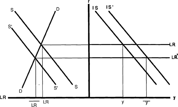
Figure 3 depicts an expansionary monetary policy using the new framework. The right-hand side of Figure 3 is the conventional IS curve in the income interest rate space. The left-hand side, shows the determination of the short-term interest rate from the intersection of demand and supply schedules for liquid reserves. The supply of liquid reserves LR_S is shown on the graph as a positive function of the interest rate.

As will be discussed below, ω is determined by policy-makers and could easily be set to zero. Notice first that the LR curve (which equates the demand and supply of liquid reserves) is horizontal, in contrast to the previous vertical LM curve. Its position is determined by open market operations which change the quantity of liquid reserves. In other words, the central bank influences a short-term interest rate which will not depend, in the short-run, on the interaction between money and output. Expansionary monetary policy will now involve shifting the LR curve down, lowering domestic short-term interest rates and, in turn, depreciating the domestic currency. The depreciation reinforces the expansionary effects on income by shifting to the right the trade balance component of the IS curve. The exact size of the response in income to a change in LR depends crucially on the size of the co-efficient β. If, as suggested above, β is very small, then the multiplier will be very large. In other words, it will take only a very small change in open market operations to cause a large change in income. Monetary policy will remain potent, even in a world without money.

It should also be pointed out that the level of LR may be highly volatile if u and ε₄ have a high variance. This variation in LR would not imply an active monetary stance, but merely reflects the role of the central bank in supplying whatever short-term liquidity is needed in the financial system to ensure its stability. Policy changes may, in fact, imply very small changes in LR relative to normal random movements in demand, so that distinguishing regular relationships between monetary policy and the economy may not be possible by looking at the relationship between LR and Y.

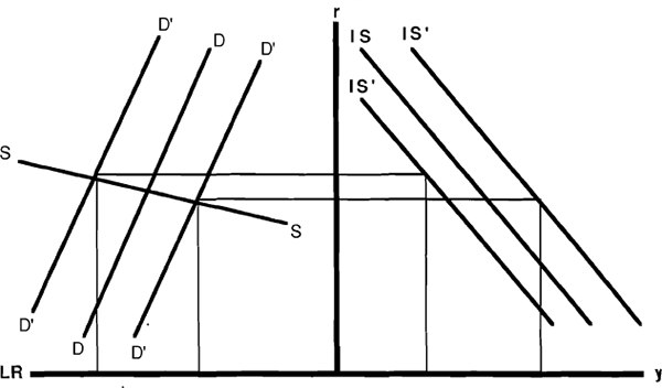
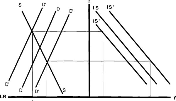
To help explain this further, the above diagrams can be extended into a stochastic framework to evaluate alternative policy rules as was first done by Poole (1970). Figures 4 and 5 provide both the stochastic IS curve in the traditional income (y) and interest rate (r) space, along with demand and supply curves for liquid reserves (LR) under alternative supply rules. Figure 4 shows the highly elastic supply curve (marked SS) normally associated with fairly close interest rate targeting. The demand curve for LR is marked as DD, with the parallel lines (marked D'D') representing the variances of the stochastic shocks hitting the demand for reserves. The optimality of this policy approach is evaluated by looking at the variance of income. With the interest rate held fixed in this policy setting the size of the variance in income is determined by the stochastic shocks hitting the goods market or IS curve.

In contrast, a move towards a reserve targeting policy, shown in Figure 5 as a steeper SS curve, introduces larger fluctuations in the interest rate and substantially raises the variance of income. The model stresses the importance of central bank policy in supplying short-run liquidity to the banking sector to ensure stability in both the financial and real sectors. This is in sharp contrast to conventional IS/LM models which give ambiguous answers on the relative merits of interest rate versus money stock control. In particular, the desirability of targeting money in the IS/LM model depended crucially on the the variance of the money demand shocks being smaller than goods market shocks (given model parameters). This ambiguity is not present in IS/LR framework which always calls for the short-run stabilization of interest rates in order to minimize the variance in income.

It is interesting to speculate on the likely demand for intermediated assets (what Tobin and others call ‘inside money’) in this perfectly deregulated system. If one continues to use the old LM equation to derive a demand for such assets, then the LM curve would shift passively to the right following a monetary expansion as financial institutions create more credit and deposits to accommodate increased transactions demand. However, it could also be argued that the LM equation is not a suitable approach to modelling the demand for intermediated assets. In a fully deregulated world, the private sector's demand for assets will reflect, more closely, their intertemporal savings decisions. For example, a policy-induced fall in interest rates makes it less attractive to save, and more attractive to spend, so there may in fact be a decline in the demand for intermediated assets following an easing of monetary policy, rather than an expansion. In any case, the stock of such assets outstanding will no longer be relevant for the implementation and transmission of monetary policy.

Footnotes

Such perfectly liquid reserves would be the equivalent of “exchange settlement funds” in Australia which are largely held as loans to dealers. In the U.S. they are equivalent to what is called “excess reserves”. [10]

In the present Australian financial system, the demand for settlement funds is also a positive function of the penalty rate charged on rediscount facilities (see Dotsey, 1987). The model abstracts from many such institutional features of the current Australian financial system in order to be as abstract and general as possible. [11]

Excess reserves in Australia (loans to dealers) receive a market related rate of interest. This implies they are even more insensitive to interest rate changes than might be expected. [12]

This appears to be the case in Australia, where the stock loans to dealers can change by over 100 per cent on a daily basis. [13]