RDP 9314: The Demand for Money in Australia: New Tests on an old Topic 3. The Data and Their Order of Integration
December 1993
- Download the Paper 135KB
3.1 The Data
The various definitions of money, income and interest rates employed in this paper are set out below. Appendix 1 contains full definitions and data sources.
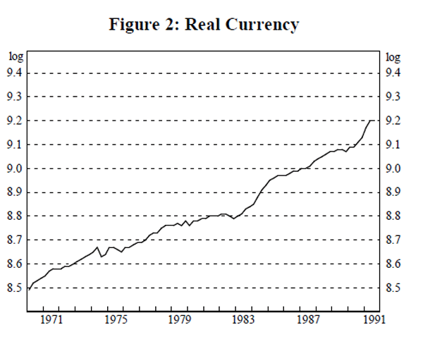
Currency is defined as notes and coins held by the non-bank private sector in Australia and, at December 1992, totalled $16.3 billion. Figure 2 shows the natural logarithm of real currency.[2]
The standard definition of the money base is the sum of notes and coins held by the private sector, plus deposits of banks with the Reserve Bank (as well as some other minor Reserve Bank liabilities to the private sector). Currency constitutes about 80 per cent of the money base, with bank deposits with the RBA making up the remaining 20 per cent. The latter comprises exchange settlement accounts and, by far the major proportion, non-callable deposits (‘required reserves’).
| Author | Dependent Variable | Independent Variables | Data and Methods | Results |
|---|---|---|---|---|
| Orden and Fisher (1993) | Nominal M3 | Real GDP, nominal 13-week Treasury note rate and GDP deflator. | Quarterly, 1965:2 to 1989:3. Variables are defined alternatively in seasonally-adjusted terms and seasonally-unadjusted terms, with seasonal dummies included in the latter case. Variables apart from the interest rate are in natural logarithms. Estimated using the Johansen (1988) procedure. | One cointegrating vector between M3, real GDP and prices only in the pre-deregulation sub-period 1965:2 to 1982:4. The result holds for either seasonal adjustment approach. |
| Lim and Martin (1991) | Real M3 (GDP deflator) | Real GDP, nominal 90-day bill rate, 2-year bond yield and 10-year bond yield and annual percentage change in the GDP deflator. | Quarterly, 1970:4 to 1990:2. Variables apart from interest rates are seasonally-adjusted. Variables apart from interest and inflation rates are in natural logarithms. Estimation method is Park's (1988) H-test. | Long run relationship between real M3, real GDP and 10-year bond yield. ECM estimated including short-term interest rate. |
| Lim (1991) | Real currency, real bank deposits and real non-bank deposits (GDP deflator) | Real GDP, real broad money, 90-day bank bill rate, 2-year bond yield, 10-year bond yield and annual percentage change in the GDP deflator. | Quarterly, 1976:3 to 1990:2 and monthly 1976:08 to 1990:06. Variables apart from interest rates are seasonally-adjusted. Variables apart from interest and inflation rates are in natural logarithms. Phillips-Hansen (1990) technique used. A structural change dummy was also included for the 1982/83 recession and for the effects of deregulation and rapid depreciation in 1985. | Long run relationships on both data sets including all variables except the bill rate. ECM estimated including bill rate |
| Lim and Dixon (1991) | Real currency (GNE deflator) | Real GNE and 3 month average of 90-day bill rate. | Quarterly, from 1977:1 to 1989:2. Variables are seasonally-unadjusted and so seasonal dummies are included. Estimation by OLS following the Engle-Granger procedure. | Long-run relationship between real currency and real GNE. |
| de Haan and Zelhorst (1991) | Real M3 and real M1 (deflated by the CPI) | Real GDP (deflated by the CPI) and 3-year Treasury bond yield. | Quarterly, from 1960:1 to 1989:2 and variables apart from the bond yield are seasonally-adjusted and in natural logarithms. Engle-Granger (1987) estimation procedure. | Long-run relationship between GDP velocity of M3 and 3-year bond yield from
1960:1 to 1983:4 only. |
| Hargreaves (1991) | Real money base and real M1 (alternatively deflated by GDP and GNE deflators) | Alternatively GDP and GNE, tax-adjusted 90-day bill rate, 2-year bond yield and savings account interest rate (with the tax rate calculated as the ratio of net household disposable income to total household income), a risk variable (the standard error on 15-year Treasury bond yields) and alternatively the quarterly change in GDP and GNE deflators. | Quarterly, from 1973:3 to 1989:4 and all variables are in natural logarithms. Variables are seasonally-unadjusted. Engle-Granger (1987) estimation procedure. | Long-run relationship between real money base and real M1 and, alternatively,
GDP and GNE and, alternatively, tax-adjusted 90-day bill rate and 2-year
bond yield. |
| Juselius (1991) | Nominal M1 and M3 | Alternatively real GDP and real GNE, alternatively GDP and GNE implicit price deflator, nominal 90-day bill rate and nominal ten-year bond yield. | Quarterly from 1975:3 to 1991:1. Variables are seasonally-unadjusted and,
apart from interest rates, are in natural logarithms. Seasonal dummies
are included. Estimated using the Johansen (1988) procedure. |
Two cointegrating vectors between money and real activity, prices, short and long-run interest rates and a time trend for each definition of money and each definition of activity. |
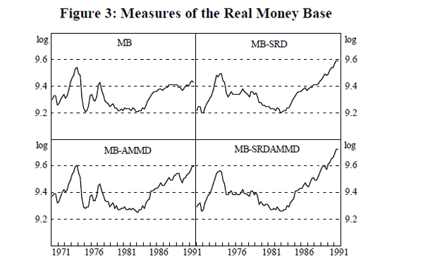
This definition, published by the Reserve Bank, is referred to in this paper as MB. There are several alternative or augmented definitions. MB-SRD refers to the standard money base adjusted to eliminate the effect of changes in the Statutory Reserve Deposit (SRD) ratio.[3] The adjustment procedure is explained in Appendix 1.
MB-AMMD adds bank loans to authorised dealers in the short-term money market to the standard definition of the money base. This recognises the fact that banks' excess reserves in the Australian system are not held at the Reserve Bank, but with the dealers. These funds are available on a ‘same day’ basis to banks, and are therefore as good as cash at the Reserve Bank. They also bear interest, in contrast to exchange settlement accounts at the RBA. MB-SRDAMMD further adjusts this definition for the SRD changes. These four definitions of money base are shown in Figure 3.
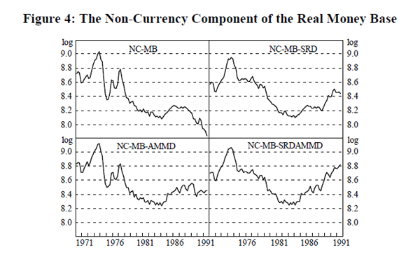
While the money base is dominated by currency, some economists regard reserves as the analytically important component of the money base and so we examine the non-currency component of the money base separately. NC-MB, NC-MB-SRD, NC-MB-AMMD and NC-MB-SRDAMMD refer respectively to the non-currency components of the above definitions of money base. These measures are shown in Figure 4.
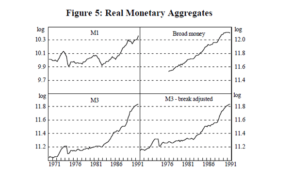
The other definitions of money used in the paper are the conventional ones. M1 in Australia has traditionally been defined as currency plus current deposits held with trading banks. Since the distinction between trading and savings banks was removed in January 1990, this aggregate is technically defunct. Accordingly, we define M1 as currency and current deposits with all banks.[4]
M3 is defined as currency plus bank deposits of the non-bank private sector. Changes in the legal status and operations of financial institutions have had a significant effect on the growth of M3 over time. The series adjusted for changes in the classification of financial institutions is called M3-BA.
Broad Money includes M3 plus borrowings from the private sector by non-bank financial intermediaries (NBFIs), less their holdings of currency and bank deposits. As a broader measure of money, it is substantially less affected by changes in financial intermediation. These last four monetary aggregates are shown in Figure 5.
Selection of the income and interest rate variables is largely an empirical matter. We test relationships across a range of definitions – gross domestic product (GDP), gross national expenditure (GNE) and private final demand (PFD), (all shown in Figure 6), and 3-month, 2-year and 10-year interest rates (Figure 7), as well as measures of own rates of return on the monetary aggregates (Figure 8). This is not ‘specification searching’[5], in pursuit of the ‘ best’ result. Rather, it is motivated by our prior that a relationship which is sensitive to arbitrary changes in specification is not particularly robust.
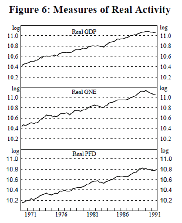
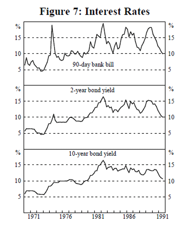
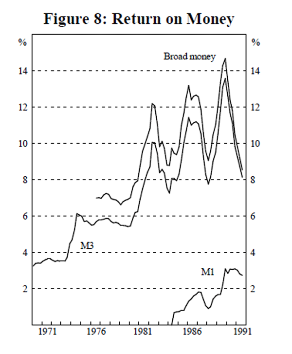
The money demand equations are estimated on a quarterly basis from the March quarter of 1970 to the September quarter of 1991, except for broad money and the broad money own-rate which are only available from the December quarter of 1976. The data, except for the interest rates and inflation rates, are expressed in natural logarithms. In accord with a substantial body of the empirical literature, the variables, apart from interest rates, are seasonally-adjusted. Using seasonally-adjusted data avoids the need to test for seasonal integration and reduces nuisance parameters. Furthermore, most of the seasonal adjustment is conducted by the Australian Bureau of Statistics using all available information, and so the seasonal adjustment is more comprehensive and accurate than that obtained by using more elementary seasonal adjustment procedures[6] or by including seasonal dummies. The results of Orden and Fisher suggest that the method of seasonal adjustment is inconsequential. If the seasonal patterns are themselves stationary, as should be the case since they have a mean of unity, then the issue of seasonal adjustment should be irrelevant to the long-run relationship between the variables.
3.2 The Order of Integration of the Data
The augmented Dickey-Fuller (ADF) test (Said and Dickey (1984)) and Zt test (Phillips (1987)) are used for determining the order of integration of the variables under consideration. The tests are initially conducted allowing for a deterministic trend in order to commence with the most general data-generating process. The results, assessed at the 5 per cent critical level, are summarised in Table 2.[7] The unit root testing procedures are outlined in Appendix 2.
| Variable | ADF | Zt | ADF after considering break in deterministic trend |
|---|---|---|---|
| Currency | I(1) | I(1) | I(1) |
| MB | I(1) | I(1) | I(0) |
| MB-SRD | I(1) | I(1) | I(0) |
| MB-AMMD | I(1) | I(1) | I(0) |
| MB-SRDAMMD | I(1) | I(1) | I(1) |
| NC-MB | I(1) | I(1) | I(1) |
| NC-MB-SRD | I(1) | I(1) | I(0) |
| NC-MB-AMMD | I(1) | I(1) | I(0) |
| NC-MB-SRDAMMD | I(1) | I(1) | I(1) |
| M1 | I(1) | I(1) | I(0) |
| M3 | I(1) | I(1) | I(1) |
| M3-BA | I(1) | I(1) | I(1) |
| Broad Money | I(1) | I(1) | – |
| GDP | I(1) | I(1) | I(1) |
| GNE | I(0)# | I(1) | I(0) |
| PFD | I(0)# | I(1) | I(0) |
| 90-Day Bank Bill Rate | I(0)# | I(1) | – |
| 2-Year Bond Yield | I(1) | I(1) | I(0) |
| 10-Year Bond Yield | I(1) | I(1) | I(1) |
| M1 Own-Rate | I(1) | I(1) | – |
| M3 Own-Rate | I(0)# | I(1) | – |
| Broad Money Own-Rate | I(0)# | I(1) | – |
| * real values for monetary aggregates presented here are deflated by GDP
deflator. # I(0) in the presence of a deterministic trend. |
|||
The unit root tests indicate that the monetary aggregates defined in real terms are integrated of order one. Real activity appears to be integrated of order one in the case of real GDP for both the ADF and Zt tests, though not necessarily for real GNE and real PFD, where the ADF tests indicate that the levels of real GNE and real PFD are stationary around a deterministic trend.
The ten-year and two-year bond yields and the estimated M1 own-rate are clearly I(1), while the bill rate, the estimated broad money own-rate and the estimated M3 own-rate are I(1) under the Zt procedure but I(0) around a deterministic trend under the ADF procedure. Given the low power of these tests in differentiating the underlying data generating process, we are inclined to treat the series as I(1).
The tests applied above are standard. Perron (1989, 1990), however, demonstrates that standard tests of the unit root hypothesis are biased toward acceptance of the null hypothesis of a unit root if the true data generating process is stationary around a trend line with one break. Perron (1989) models a break in the trend level, a break in the trend slope and a combination of the two and estimates critical values for unit root tests for each of these models. This is relevant to the present study: even a summary glance at Figures 2 to 5 of the real monetary aggregates shows that many of the series appear to contain at least one break in the level or in the slope of its trend. The limitation of Perron's method is that it is properly applied only when the date of the break is known and when there is only one break. We determine break dates by inspection of the series and then suggest reasons for the break. The results are summarised in the final column of Table 2.
Evidence of stationarity around a broken trend is found only for the money base variables and M1. The break in the money base occurs in 1982/83 in the reserve deposit component. The accelerated growth in SRDs is due to the rise in fixed deposits and certificates of deposit as banks were freed from regulation and were able to compete for funds in an economy undergoing a strong recovery. M1 may also be modelled as a stationary process around a deterministic time trend but with a single break in the slope occurring some time in 1985 or 1986. This coincides with the removal of the restriction of the payment of interest on current deposits in August 1984.
For both the money base and M1, there are a number of possible break dates, almost all of which yield the same result that the aggregate is I(0) around a broken trend, suggesting that the results are not mere chance outcomes. The other aggregates remain I(1), though most of the selected trend breaks appear to be significant.
In terms of cointegration analysis, if the money base and M1 are I(0) processes around a broken trend, then, strictly speaking, the analysis stops there: money and income are not integrated of the same order and so cannot be cointegrated. There are, however, two alternatives:
- it still makes sense to talk of a relationship between the time series examined if income and interest rates are also I(0) around a broken trend. Perron tests were applied to these series but they do not appear to be I(0) processes around a broken trend, with the exception of GNE, PFD and the two-year bond yield, the break in the latter coinciding with the shift in the early 1980s from a tap to tender system for government bonds; or
- given that unit root tests on the whole have weak power in identifying the true statistical properties of the data series, and that cointegration methodology is still in its infancy, it may be legitimate to treat the money base variables and M1 as I(1) processes.
We proceed on the basis of the second alternative.
Footnotes
In the graphs which follow, the various monetary aggregates are deflated by the implicit GDP price deflator. By convention, one billion is defined as a thousand million. [2]
Before 1981, the SRD ratio was varied as a monetary policy instrument. A tightening of policy by increasing the SRD ratio would mechanically increase the money base, giving a signal contrary to that expected of demand for an asset. [3]
Current deposits placed with savings banks can be identified only from February 1975 and so there is a small break in M1 at this time. [4]
See Cooley and LeRoy (1981). [5]
As explained in Appendix 1, the seasonally-adjusted M1, M3 and break-adjusted M3 series are spliced at February 1975. Our judgment is that splicing two ABS seasonally-adjusted series to obtain one seasonally-adjusted series is preferable to using a seasonal adjustment procedure such as X-11Q to deseasonalise the longer unadjusted data series. [6]
Full details of all results reported in this paper are available from the authors on request. The lag ordering is set so that the residuals in the ADF test equation are not serially correlated (based on the Lagrange multiplier test). A constant and time trend are included only if statistically significant at the 5 per cent level. The lag ordering for the Zt test is set arbitrarily at 5 and 10. [7]