RBA Annual Conference – 1992 The Great Inflation, The Great Disinflation, and Policies for Future Price Stability John Taylor[*]
1. Introduction
With underlying inflation rates in the United States and many other countries now reaching levels not seen since the early 1960s, a remarkable history of a great inflation and an equally great disinflation is concluding. This history is worthy of study from many perspectives. From an economic perspective, the history raises profound theoretical, institutional, empirical and causal questions. It involves the development and serious application of new macro-economic theories – from Keynesian economics to rational expectations. It includes major changes in the institutions of policy making – from the demise of Bretton Woods to the development of the European Monetary System. It is related, in the view of many analysts, to changes to demographic and geopolitical factors – from the post World War II baby boom to the oil price changes emanating from political developments in the Middle East. It provides an opportunity to observe influential policy makers – such as Walter Heller and Paul Volcker in die United States – in action. And it demonstrates the colossal effects of inflation on economic well-being – generating large transfers of income, causing recessions and financial strains, some relating to the Saving and Loan crisis in the United States, and affecting politics more generally.
This paper begins with a brief review of that history. However, the main aim of the paper is prospective, not retrospective. By combining the lessons of that history with recent results in time series analysis and econometric policy evaluation, I endeavour to draw implications for the design and operation of monetary policy to maintain price stability in the future.
The paper is organized as follows. In Section 2, I review several recent historical studies of the great inflation – disinflation period. These studies provide a consensus on the pattern of inflation and the role of monetary policy; they also outline possible underlying causes of the inflation and disinflation. In Section 3, I examine the empirical relationship between price and output dynamics – so important for the study of policies to achieve price stability, and, using vector autoregressions, I show that this relationship has remained remarkably stable since the mid-1980s. In the late 1980s we still find counter-clockwise loops in inflation-output scatter diagrams, much as we did in the 1960s and 1970s. I also examine the monetary tightening in the United States, Germany and Japan in the late 1980s in order to understand why the business cycles seem out of synchronization in the early 1990s, unlike the early 1980s. In Section 4, 1 report on recent research – including my own – on the design of monetary policy rules to keep price and output fluctuations low.
2. Inflation, Disinflation and the Proximate Causes
Some of the recent studies that have reviewed the inflation – disinflation history of the last 30 years include Bomhoff (1991), Dornbusch and Fischer (1991), Friedman (1992), Fry (1991), Lebow, Roberts and Stockton (1992), Parkin (1991), Stevens (1991) and Ueda (1991). Although there are important exceptions, which will be noted below, a general pattern emerges from many of these studies. Inflation began to rise starting in the mid-1960s, continued to rise through the late 1970s, declined sharply in the early 1980s, remained steady through most of the 1980s and then began to decline again in the early 1990s. There are differences in the level of inflation in different countries, but this general time series pattern is surprisingly common.
Parkin (1991) focuses on the United States and Canada. He documents the gradual, upward movement in inflation in the 1960s and 1970s in both the United States and Canada, and the rather abrupt decline in the early 1980s. Inflation then held steady in the 4 to 5 per cent range through most of the 1980s. Although the early 1990s are beyond Parkin's sample period, it is now clear that a further reduction in inflation has occurred. The last few years in the United States have seen the second installment on a disinflation from the high level of the 1970s. The Fed lowered the midpoint of its targets for money growth (M2) from 7 per cent in 1987 to 4½ per cent in 1991. Assuming no long-run trend in velocity, and given a growth rate of potential output of 3 per cent this implies a reduction in the inflation target from 4 per cent to 1½ per cent, very close to price stability. Although not quite that low now, inflation is lower than it has been since the early 1960s, before the run up in inflation in the mid-1960s.
Bomhoff (1991) shows that the same general time series pattern fits most of the countries of Western Europe. As with the United States and Canada, inflation rose in the 1970s and significant disinflation occurred in the early 1980s. However, in some countries of Europe, especially Germany, inflationary pressures have remained strong in the early 1990s and there is little evidence yet of further disinflation. In addition to tracing out similar patterns in the G7 countries, Lebow, Roberts and Stockton (1991) look for subperiods of low inflation and inflation stability. They find very few: the 1950s and early 1960s in 4 of the G7 countries – the United States, Germany, Canada, and France. Japan, Italy and the United Kingdom do not pass the low inflation-stable inflation test in this period, although Japan does in the 1980s.
Fry (1991) studies eight Pacific Basin countries – Malaysia, Thailand, Singapore, Hong Kong, Indonesia, Taiwan, Korea and the Philippines – and presents a history of inflation and disinflation which is, on average, remarkably similar to the developed countries, including a relatively stable inflation rate in those countries during much of the 1980s. Stevens (1991) examined the experience of Australia and presents the same general pattern, although, as he emphasizes, the approximately 7 per cent inflation rate throughout much of the 1980s was higher than the G7 average. More recently, the rate of inflation in Australia has taken another downward step and is around 3 per cent in mid-1992.
Dornbusch and Fischer (1991) examined eight countries – Chile, Mexico, Columbia, Brazil, Korea, Indonesia, Ireland and Spain. The Pacific Basin and Western European countries in their group show the same pattern documented by Fry and Bomhoff. However, the Latin American countries studied by Dornbusch and Fischer are significant exceptions to the general pattern of disinflation followed by relatively low inflation in the industrialized countries in the 1980s and early 1990s. They are still in the high-inflation range, a reminder that high inflation has not yet disappeared from the face of the Earth. In addition, high inflation remains a problem in the economies in transition in Eastern Europe and the former Soviet Union.
Japan is another kind of exception to the general pattern of inflation and disinflation. As documented by Ueda (1991), the high inflation in Japan ended in the mid-1970s rather than the early 1980s as in the other countries. And it stayed at a relatively low and stable rate through the late 1980s. Japan is the only G7 country to have stable inflation for long enough to pass the Lebow, Roberts and Stockton (1991) test in recent years.
(a) Money Growth as a Source of Inflation
What does the empirical evidence suggest was the proximate cause of this inflation and disinflation? Friedman (1992) reviews the history of money growth and inflation in the United States, the United Kingdom, Germany, Japan and Brazil and documents a strong correlation between money growth and inflation. Parkin (1991) argues that changes in the money supply were the dominant source of inflation in the United States and Canada. Bomhoff (1991) describes strong money-price correlations in his study of Western European countries and Fry (1991) reports similar results for the Pacific Basin countries.
To be sure, increases in the price of oil in the 1970s were related to some of the bursts of inflation, but these would not have been sustained without monetary accommodation. The experience of Japan during the 1979 oil shock – when inflation did not take off as in the rest of the OECD, and the experience of most of the other OECD countries during the oil shock of 1990, when inflation did not take off – is strong evidence on this point. In general, there is ample evidence in many of the recent experiences with inflation and disinflation to support Friedman's (1992) point that ‘substantial inflation is always and everywhere a monetary phenomenon.’
(b) Concerns About the Stability of Money Demand
Despite the importance of money in explaining inflation, there are still legitimate concerns about the stability of money demand, especially in the short run. To be sure, in some countries money demand appears to be fairly stable. For example, Fry (1991) performed tests for structural stability that showed a surprising amount of money demand stability in the eight Pacific Basin countries that he looked at. But structural stability tests have very weak power unless the underlying equations fit the data very well. Bomhoff (1991) also found stability of money demand in Western Europe using the Kalman filter technique. Despite these studies, direct experience with the use of money aggregates for guiding monetary policy in the short run has caused problems. In the United States, for example, the demand for narrow money (M1) went through substantial shifts in the 1980s, and the demand for broad money (M2) provided very confusing signals in the early 1990s. Similar money demand stability questions have affected monetary policy in other countries, for example, Australia, France and the United Kingdom. Also, there is concern that continued technological changes and regulatory changes will affect the demand for money in the future.
For these reasons many central banks have begun to place more emphasis on interest rates in their operating strategies in the 1980s and early 1990s. Focusing on interest rates for short-run determination of monetary policy does not, of course, mean that central banks have become less concerned about inflation. The evidence that the large swings in inflation are related to money growth indicates, however, that money should continue to play an important role in monetary policy formulation in the future. However, interest rates are likely to remain the preferred operating instrument of monetary policy.
(c) Underlying Causes
Friedman (1992, p. 193) states that ‘the recognition that a substantial inflation is always and everywhere a monetary phenomenon is only the beginning of an understanding of the cause and cure for inflation. The more basic questions are: Why do governments increase the quantity of money too rapidly? Why do they produce inflation when they understand its potential for harm?’
Or in terms of the history of the last 30 years, why did governments allow inflation to increase in the 1960s and 1970s and then reverse their policies in the early 1980s? Why was there another attempt to disinflate in many countries in the early 1990s? In thinking about the lessons of inflation and disinflation for the future, this is the key question to address. In my view, there are three alternative answers.
Parkin (1991) suggests the first. He argues that the rise and subsequent fall of inflation in the United States and Canada could be due to the time inconsistency problem originally formulated by Kydland and Prescott (1977). If policy makers cannot commit themselves to a policy, they may get stuck in a sub-optimal high-inflation equilibrium. In the Kydland and Prescott model, prices are perfectly flexible and expectations are rational, so there is no short-term trade-off between inflation and unemployment. Hence, the optimal policy yields price stability with the unemployment rate always equal to the ‘natural’ (non-inflationary) rate. For the non-optimal policy, however, the higher is the natural rate of unemployment, the higher is the rate of inflation in the sub-optimal equilibrium. Parkin's (1991) argument is that policy makers are always in a sub-optimal equilibrium. However, that equilibrium changes when the natural unemployment rate changes. Hence, the time series pattern of inflation might be explained by a time series pattern of the natural rate of unemployment, which has rough similarities to the movement of inflation.
In fact, most estimates suggest that the natural rate of unemployment did rise in the United States in the 1960s and 1970s, partly because of the entrance of the baby boom generation into the labour force. And, as the number of young entrants into the labor force declined in the 1980s, so has the natural rate of unemployment. Hence, these demographic changes could have been the source of the inflation and disinflation process.
The second explanation places more emphasis on the impact of economic research and changes in the perceptions of how the economy works. In the early 1960s the consensus macro-economic model was much different from the consensus model today. The models popular in the early 1960s claimed that there was a permanent negative trade-off between the level of unemployment and the level of inflation. Today almost no model predicts that. The increase of inflation in the 1960s and the 1970s could have been due to these faulty inflation-unemployment models. They were actively put forth in policy-making circles in the United States, including the Council of Economic Advisers, in the 1960s. But, if there is any change in the paradigm of macro-economics that most economists would agree with, it is that the trade-off view was mistaken.
Faulty estimates of the cost of inflation could also have been a factor. Economists seem to have underestimated the cost of inflation, at least compared to assessments in public opinion polls. By the late 1970s the costs of inflation were perceived to be higher than was previously thought. Moreover, lower estimates of the costs of disinflation came to be more widely accepted, especially with the increased emphasis on credibility and rational expectations. Those factors could explain the rise and subsequent fall of inflation. Similar changes in the intellectual underpinnings of policy occurred in the United Kingdom in the late 1970s and the early 1980s, and presumably in other countries.
The third explanation is related to a traditional role of money creation: inflationary finance, as frequently observed during wars, or when it is difficult to raise government revenues through a conventional tax system. Clearly inflationary finance is a significant factor in the Latin American inflations.
In the United States inflationary finance in the traditional sense has been very small during the 1960–1990 period. The monetary base was about $325 billion in the United states in 1991. An increase in the inflation rate of 10 percentage points would raise ‘tax’ receipts by only $33 billion per year, even assuming no reduction in money demand. This compares with actual tax revenues of $1,100 billion per year, and equals only 3 per cent of such revenues. It is difficult to believe that the inflation increase in the 1960s and 1970s would have been undertaken for this small amount. The optimal tax literature views the inflation tax as one among many taxes; the optimal tax mix incorporates the inefficiencies of each tax. However, there is little evidence that the efficiency of conventional tax collection declined in the 1970s and increased in the 1980s in the United States.
Inflation can affect government financing in other ways. An unanticipated increase in inflation reduces the outstanding value of government debt, and, if the tax system is not indexed, provides a hidden tax increase through bracket creep. Neither of these factors seems capable of explaining both the rise and fall of inflation in the 1960–90 period. During the 1970s the debt to GNP ratio was at a post-War low in the United States, and the personal tax system was indexed after the disinflation of the early 1980s. Hence, the elimination of the bracket creep motivation for inflation came too late to explain the disinflation.
In my view the second of these three explanations is most satisfactory. As I have already indicated, the inflationary finance argument has difficulty explaining both the increase in inflation and the disinflation. And, as I have argued elsewhere (Taylor (1983)), using the time-inconsistency argument as positive economics requires the world to behave according to a model with perfectly flexible prices in which everyone knows that such a model is correct, and in which there are no institutions to maintain the optimal monetary solution. In other areas where time inconsistency is a potential problem, such as patent law, we have designed institutions to handle the time-inconsistency problem. We do not repeal the patent laws every time there is an invention in order to eliminate the inefficiency of monopoly.
Whichever answer one chooses, however, there does seem to be some hope that a repeat of the inflation-disinflation history will be unlikely in the future. Many of the forces that may have led monetary policy makers to permit the great inflation of the 1960s and 1970s have diminished. There is no projected increase in the natural rate of unemployment even with a small echo effect of the post-War baby boom. There is no evidence that current economic research is likely to revive a negative long-term relationship between the level of inflation and the level of unemployment (at least for positive levels of inflation). Indexing and lowering of the personal income taxes (in the United States at least) makes bracket creep less significant. To be sure, the level of debt to GDP is higher now in the United States than it was in the 1970s and, after stabilizing in the late 1980s, is rising again. However, it is still well below the level of the 1950s and early 1960s, when we had relative inflation stability.
Although there is some consensus that low inflation or price stability is more desirable than in the past, there is not consensus about what low inflation means. There is agreement that the upward bias in the measurement of inflation appears to be relatively small, perhaps in the area of 1½ per cent or 2½ per cent. See Gordon (1991) or Fortin (1990). But there is not a complete agreement, at least among economists, that 1½ to 2½ per cent inflation is a good target. For example, Fischer (1991) expressed the view that low inflation could be around 4 per cent. On the other hand, research reported in Lipsey (1990) suggests that it is unlikely to be that high.
In any case, it appears that in many countries monetary policy can focus more attention in the future on maintaining the price stability that has been achieved. However, it is not safe to say that a world without substantial inflation and disinflation will be free from recessions or growth cycles. In fact, without a firm indicator of the impact of monetary policy, it is clear that monetary cycles will remain and that monetary authorities will continue to face short-term trade-offs between inflation and output. Clearly the most pressing task is to find good rules for monetary policy – probably with the interest rate as the instrument – that reflect such trade-offs. Issues relating to that task are what I address in the remainder of the paper.
3. The Relationship Between Inflation and Output
An understanding of the relationship between inflation and output fluctuations is essential to designing policies to maintain price stability. Yet there is still considerable debate among macro-economists about such fluctuations. The idea of rational expectations has become dominant in academic research, but there is still a split between those who assume and utilize the assumption of sticky prices and other rigidities and those who maintain the perfectly flexible price assumption.
In the United States, for example, the real business cycle view, in which prices are perfectly flexible and money does not play a role in the cycle, is a subject of advanced research by many academic economists. From the perspective of formulating monetary policy, however, the real business cycle model is by definition inadequate; it does not include monetary policy, and it does not explain the strong correlation between price and output fluctuations evident in the data. Future modifications of the real business cycle model may indeed incorporate money and explain the link between output and price fluctuations. Indeed, Christiano and Eichenbaum (1992) and Coleman, Giles and Labadie (1991) have already made advances in that direction. In the meantime, however, models that incorporate some degree of price rigidities along with rational expectations are better able to explain the facts relevant to designing and choosing a policy for maintaining price stability.
Tables 1 through 3 address the issue by presenting time series evidence on inflation and output fluctuations. I focus this empirical work on quarterly data from the OECD Quarterly National Accounts for the United States, Germany and Japan. The three tables show the coefficients of simple bivariate vector autoregressions of inflation (the first difference of the log of the output deflator) and real output (measured as the percentage deviation from a trend over the 1972Q4–91Q3 period). To keep the econometrics as simple as possible, I focus on this bivariate system and include only two lags of each variable. The general findings are not changed by the inclusion of more lags.
| INF(−1) | INF(−2) | GDP(−1) | GDP(−2) | S.E. | RES AC | CHOW | EXOG | |
|---|---|---|---|---|---|---|---|---|
| INF | 0.368 [0.103] |
0.518 [0.105] |
0.09 [0.045] |
−0.052 [0.046] |
0.004 |
−0.076 |
3.65 |
|
| 1.05 | ||||||||
| 0.321 [0.121] |
0.494 [0.122] |
0.087 [0.053] |
−0.037 [0.055] |
0.004 |
−0.061 |
3.47 |
||
| GDP | −0.284 [0.251] |
0.005 [0.256] |
1.277 [0.111] |
−0.374 [0.111] |
0.009 |
−0.043 |
1.38 |
|
| 0.46 | ||||||||
| −0.346 [0.301] |
−0.001 [0.304] |
1.23 [0.132] |
−0.321 [0.304] |
0.01 |
−0.028 |
1.15 |
||
| ‘Correlation of residuals (full sample, truncated sample): 0.110, 0.094’ First line are coefficients for period 1972:4–1991:3; second line for period 1972:4–1986:4. RES AC is the first order autocorrelation of the residuals from the regressions. CHOW is the test statistic from performing a Chow test of parameter stability; EXOG is the test statistics for Granger causality. Standard errors in parentheses. | ||||||||
| INF(−1) | INF(−2) | GDP(−1) | GDP(−2) | S.E. | RES AC | CHOW | EXOG | |
|---|---|---|---|---|---|---|---|---|
| INF | 0.215 [0.107] |
0.425 [0.104] |
0.115 [0.057] |
−0.059 [0.061] |
0.003 |
−0.16 |
6.24 |
|
| 1.85 | ||||||||
| 0.212 [0.126] |
0.424 [0.120] |
0.163 [0.065] |
−0.113 [0.069] |
0.004 |
−0.136 |
5.02 |
||
| GDP | −0.146 [0.210] |
−0.331 [0.203] |
1.28 [0.111] |
−0.31 [0.120] |
0.007 |
−0.067 |
2.33 |
|
| 1.09 | ||||||||
| −0.089 [0.244] |
−0.231 [0.232] |
1.32 [0.127] |
−0.383 [0.134] |
0.007 |
−0.078 |
0.73 |
||
| ‘Correlation of residuals (full sample, truncated sample): −0.095, −0.208’ First line are coefficients for period 1972:4–1991:3; second line for period 1972:4–1986:4. RES AC is the first order autocorrelation of the residuals from the regressions. CHOW is the test statistic from performing a Chow test of parameter stability; EXOG is the test statistics for Granger causality. Standard errors in parentheses. | ||||||||
| INF(−1) | INF(−2) | GDP(−1) | GDP(−2) | S.E. | RES AC | CHOW | EXOG | |
|---|---|---|---|---|---|---|---|---|
| INF | 0.445 [0.109] |
0.364 [0.105] |
0.101 [0.099] |
0.049 [0.106] |
0.007 |
0.125 |
4.37 |
|
| 3.13 | ||||||||
| 0.46 [0.129] |
0.261 [0.121] |
0.149 [0.110] |
0.109 [0.120] |
0.007 |
0.1 |
7.47 |
||
| GDP | −0.169 [0.129] |
0.016 [0.125] |
0.938 [0.118] |
−0.011 [0.126] |
0.008 |
−0.037 |
1.78 |
|
| 0.92 | ||||||||
| −0.205 [0.159] |
0.084 [0.150] |
0.967 [0.137] |
−0.057 [0.148] |
0.009 |
−0.05 |
1.03 |
||
| ‘Correlation of residuals (full sample, truncated sample): 0.006, 0.060’ First line are coefficients for period 1972:4–1991:3; second line for period 1972:4–1986:4. RES AC is the first order autocorrelation of the residuals from the regressions. CHOW is the test statistic from performing a Chow test of parameter stability; EXOG is the test statistics for Granger causality. Standard errors in parentheses. | ||||||||
The two equations clearly show the inter-relationship between inflation and output. Technically, real output deviations are positively correlated with future inflation, and inflation is negatively correlated with future real output deviations.
These same regressions were reported in Taylor (1989) for a sample from 1972Q4 through 1986Q4, and are reported here with revised data for that same sample. Hence, the regressions in Tables 1, 2, and 3 show how these equations have changed with five additional years of data. Is there a reason to change one's thinking about the relationship between inflation and output? To be sure, there are reasons to expect some changes in these types of vector autoregressions. The earlier sample period included much of the inflation and subsequent disinflation discussed in Section 2. The last 5 years saw a combination of lower more stable inflation and more credible monetary policies. These policy changes would presumably cause shifts in reduced-form parameters. On the other hand, the later period does have a business cycle which is similar to previous cycles, in that economic policy makers attempted either to disinflate the economy or to prevent a rise in inflation.
Surprisingly, tests for structural stability (shown in Tables 1, 2 and 3) indicate little evidence of a change in the parameters in the later period. Only in the case of the inflation equation for Japan is there a statistically significant shift in the parameters, and this appears to be related to higher coefficients on the lagged value of real output. The sign and general pattern of the effect is preserved.
The infinite moving average representations of these vector autoregressions give a more visual impression of the inflation and output dynamics. These can be computed directly from the autoregressions (see Taylor (1989)), and are shown in Figures 1, 2 and 3 under the title Impulse Response Function. The top panel of each figure shows the impact on inflation of a shock to the inflation equation and a shock to the real output equation. The bottom panel shows the impact on real output of shocks to the same two equations. (The analogous infinite moving average representations for the United States and Japan are shown in Figure 3 of Taylor (1989) for the period from 1972Q4 to 1986Q4).
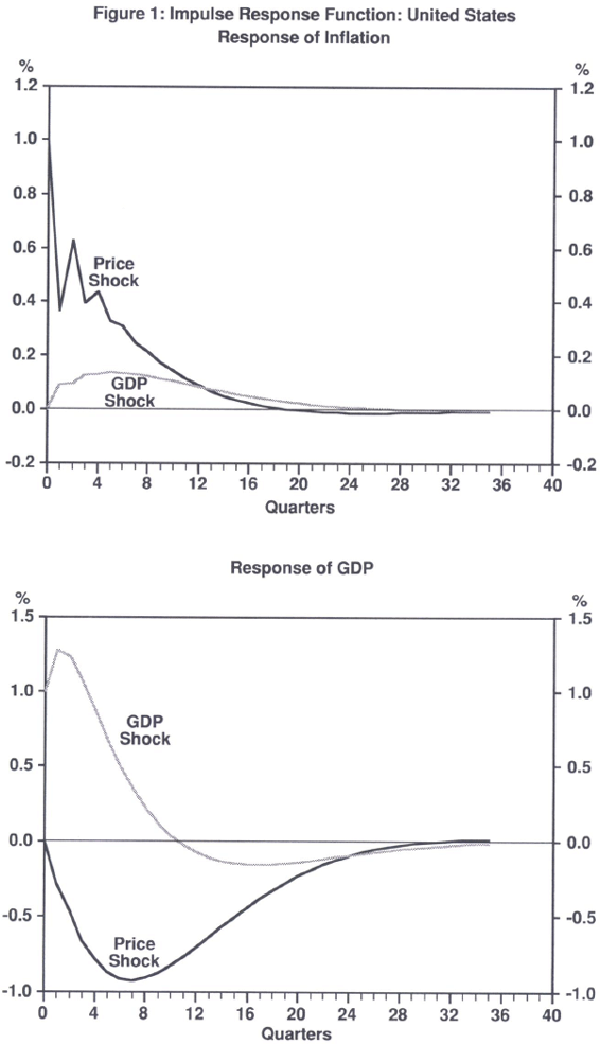
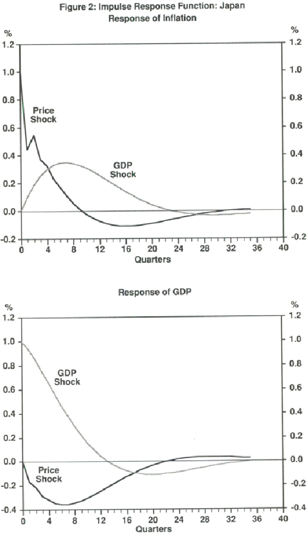
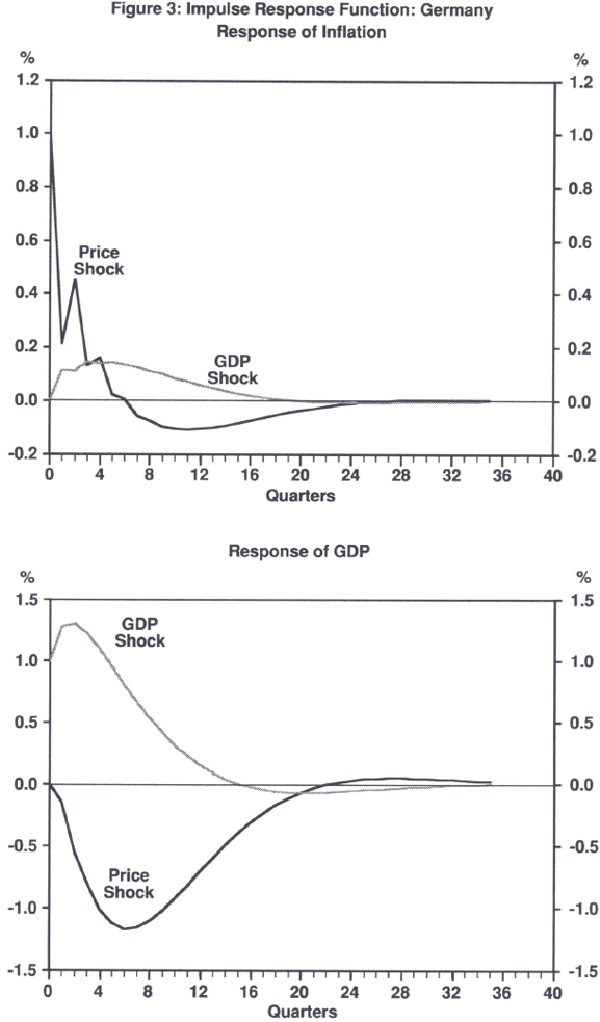
Note that the United States, Germany and Japan all have infinite moving average representations with the same general pattern. Most importantly, shocks to the inflation equation lead to declines in real output, while shocks to the output equation lead to increases in inflation. This reverse dynamic is evident in all three countries, and corresponds to the findings in Taylor (1989).
The regression coefficients in the tables and the infinite moving average representations in the figures are analogous to simple correlations. They are not themselves structural relationships; rather they are reduced forms of some structural relationships. Moreover, they do not identify any single structural interpretation.
The structural interpretation I have favoured involves a macro-economic model with sticky prices and rational expectations (see Levin (1991), Fuhrer and Moore (1989) or Taylor (1989) for discussions of more formal models). The underlying intuition that underlies these models can be simply explained. The deviations of real output from trend are interpreted as demand fluctuations – the trend in output is potential output, and positive deviations represent periods of excess demand when there are upward pressures on prices. These upward movements in demand cause, with a lag, inflation to rise, which shows up in the infinite moving average representations as positive coefficients. The lag is due to slow adjustment of wages and prices, which may be due to staggered wage and price setting. This empirical correlation corresponds to the short-run trade-off between output and inflation that is in the macro-economic data, and which therefore still needs to be in macro-economic models. The bivariate representation cannot reveal what initiated such a shock to output; the impulse could come from an unanticipated increase in the money supply or some other aggregate demand shock.
The other cross correlation shows that shocks to inflation lead to a decline in real output. The interpretation of this is that the monetary authorities do not fully accommodate inflation increases – that is, money growth is not allowed to increase as much as inflation. Hence, real money balances decline, interest rates rise and real output falls. Since the impact of money occurs with a lag, the effects are drawn out over time as shown in the figures. Of course, there are many important details about the workings of monetary policy and the persistence of inflation that are left out of this explanation and have to be provided in a formal structural model. Many of these important details remain unsettled and are the subject of current research. For example, Fuhrer and Moore (1991) argue that staggered wage or price setting must be formulated in real terms, not nominal terms, to adequately explain the persistence of the inflation shocks in Figures 1, 2 and 3. And, more generally, the microfoundations of wage and price stickiness need to be better established. Nevertheless, there is considerable agreement that this general type of model explains the data and makes sense. Caballero and Engle (1992) have recently developed a model where the micro-economic rigidities generate aggregate dynamics without all the restrictions of the staggered wage model.
The reverse dynamic correlations shown in the infinite moving average representations correspond to the counter-clockwise loops commonly used to explain the relationship between output and inflation in elementary texts. The loops are shown on scatter diagrams with inflation on the vertical axis and output on the horizontal axis. When output rises above normal, inflation rises and inflation-output pairs show a movement first to the northeast and then, as monetary policy begins to tighten, to the northwest in the scatter diagram. Eventually, output falls below normal and inflation then starts to fall tracing out points in a southwest direction and then, as policy begins to ease, in a southeast direction.
That these general correlations have remained in the data during the last five years suggests this same type of model is still appropriate for policy analysis in the future, even after price stability has been reached. To provide further evidence, I examine the actual path of inflation and output in the United States, Germany and Japan during these five years. The scatter diagrams described in the previous paragraph provide a convenient visual representation for this examination.
Figures 4, 5 and 6 show pairs of inflation and output observations from the fourth quarter of 1986 through the third quarter of 1991. About three quarters of a loop is traced out during this period in each country. And in each case the points along the loop are moving in a counter-clockwise direction. The loops are out of phase, however, as discussed below. It should be emphasized that while the points still move along the loop in a counter-clockwise direction, the loops are much smaller than the loops observed in the 1970s and 1980s, when the substantial inflation and disinflation was occurring.
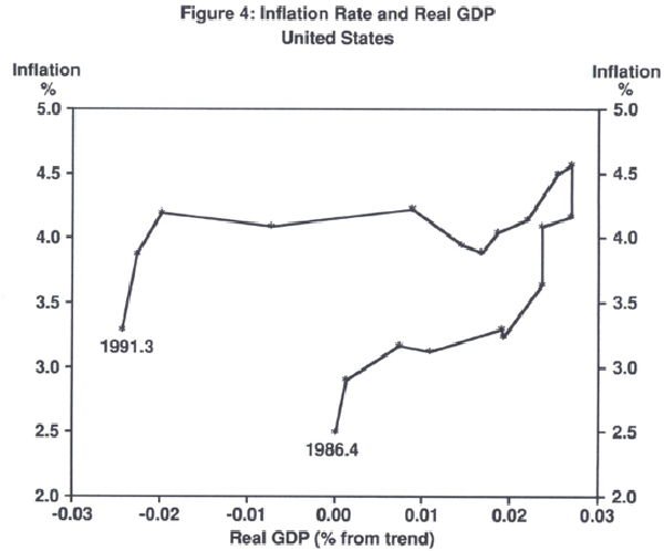
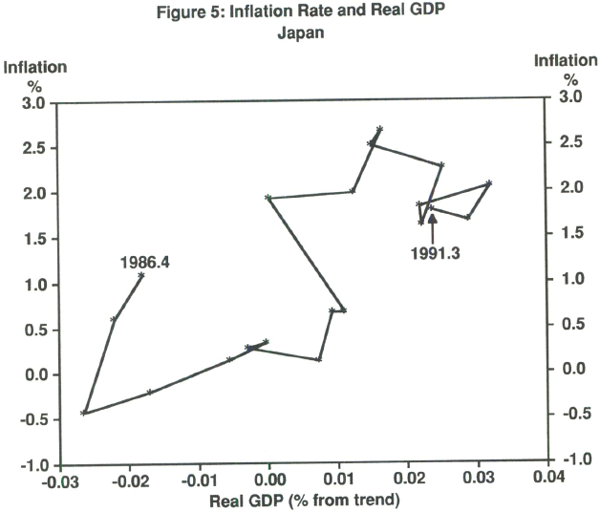
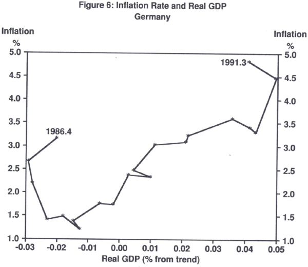
Figure 4 for the United States shows the rise of inflation and the boom in the economy in 1987 and 1988. Monetary tightening, which began in the Spring of 1988 began to have an effect in slowing the economy down by late 1989, and soon there was a decline in inflation. But, perhaps because of the rise in oil prices in the late Summer and Fall of 1990, the decline in inflation (at least by this measure) did not begin in earnest until 1991.
Figures 5 and 6 show the scatter diagrams for Germany and Japan. The data for Germany (these data do not include the former East Germany either before or after unification) still show movement in the direction of higher inflation and have only recently shown declines in output. German monetary policy was tightened later than in the United States, and aggregate demand was stimulated by the rising budget deficit associated with the unification of Germany. The data for Japan mostly reveal the boom of the late 1980s and early 1990s and the increase in inflation. Japan, like Germany, tightened monetary policy more than a year later than the United States.
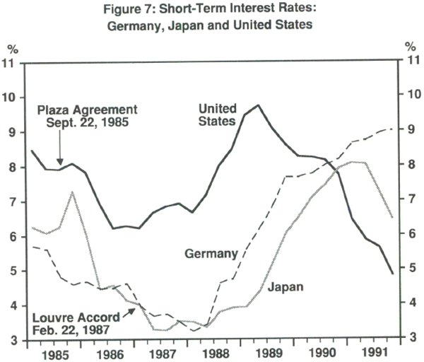
Figure 7 provides some evidence that might explain why the cyclical movements in Japan and Germany were delayed relative to the United States. The diagram shows short-term interest rates in the United States, Germany and Japan from 1985 through the first three quarters of 1991. The tightening of monetary policy in the United States in the 1987–88 period is clear, as is the delay in the tightening of monetary policy in Japan and German compared with the United States. One possible explanation for this difference, which ultimately led to the business cycle being out of synch in these three countries, was the concern about exchange rate behaviour following the Louvre Accord in February 1987. During that period there was concern that the dollar might fall further against the yen or the mark. (It had already fallen dramatically since early 1985.) If interest rates in Germany and Japan remained steady while United States interest rates rose, then yen and mark assets could be made less attractive compared to the dollar. Evidently such a concern was on the minds of monetary policy makers in these countries, and may indeed explain the delayed pattern of monetary tightening. If that delay was a mistake, then the episode indicates some remaining problems with using domestic monetary policy to achieve exchange rate goals among the G7 countries.
4. Designing and Operating Monetary Policy Rules
The preceding two sections have endeavoured to argue that the forces for a revival of a substantial inflation in the developed economies in the future have diminished, that monetary policy should be designed in the future to keep price and output fluctuations low, and that events in the last few years have not given us reason to change the basic theory of inflation and output dynamics that emerged in the 1970s and 1980s. That theory involves both rational expectations and price rigidities. It implies a significant role for monetary policy, with the details differing from model to model. This section reviews recent research which has attempted to use such models to examine the design of monetary policy.
In examining policy research during the last several years I have been struck by the large amount of work that has been devoted to finding good policy rules for monetary policy using estimated structural econometric models. Much of this research involves stochastic simulation of estimated multicountry models with rational expectations. A soon-to-be published book edited by Ralph Bryant and others (1992) at Brookings tries to bring much of this research on multicountry models together, and to compare and contrast it in a useful way. Not all recent research uses multicountry models, however. For example, Fuhrer and Moore (1991) and Lebow, Roberts, and Stockton (1992) examine strategies for monetary policy in models for the United States economy. I begin with their research.
Models that incorporate a short-run trade-off between inflation and output and that also incorporate uncertainty due to unanticipated shocks (some due to inevitable monetary policy mistakes), imply a permanent trade-off between the variability of inflation and the variability of output. This is a general feature of such models; the shape and the location of the trade-off itself depends on the model and the estimated parameters. The trade-off can be calculated by inserting a monetary policy rule into the model and seeing how it works in terms of the variability of output or the variability of inflation. Altering the parameters of the rule – say by changing the degree of responsiveness of the interest rate to the deviation of the price level from a target price level – generates different outcomes.
Tracing out these different outcomes as a function of the policy rule parameter results in the trade-off curve.
Figure 8 gives some examples of such trade-offs for the United States, as estimated by three different research groups with three different models at different points in time. The two most recent trade-off curves were computed by different researchers on the staff of the Federal Reserve Board. The trade-off labeled ‘A’ is due to Lebow, Roberts and Stockton (1992) using a small model of the United States economy with sticky prices and rational expectations. The trade-off curve labeled ‘C’ is calculated by Fuhrer and Moore (1992) using another model of the United States with rational expectations and sticky prices. The third trade-off curve, labeled ‘B’ was calculated by Taylor (1979) using yet another model of the United States with rational expectations and sticky prices, and estimated with data only through the mid-1970s. Unlike the later studies, this earlier calculation does not include data from most of the great inflation and disinflation period.
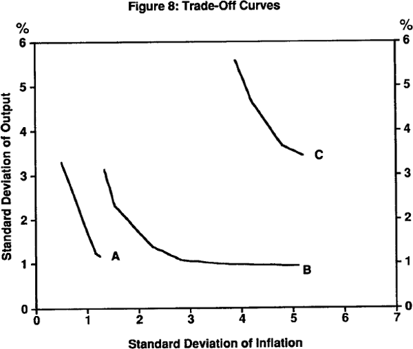
All three trade-off curves are negatively sloped with the standard deviation of the percentage deviation of output from trend on the vertical axis and the standard deviation of the inflation rate on the horizontal axis. The curves try to show graphically the trade-off that monetary policy makers face in achieving the goal of price stability. Most noticeable about these curves is that they seem so different. If it were not for the fact that the later two curves (A and C) – estimated over nearly the same sample – showed most of the difference, one might be tempted to conclude that this trade-off is as unstable as the old long-run Phillips curve trade-off. Instead, the differences reflect different modeling strategies and suggest the need for research to explain why the differences are so large; one possibility is a different assumption about information available to the monetary authorities, or about how effectively the monetary authorities can offset shocks such as shifts in money demand.
Despite the differences, however, the curves do have an important feature in common. Aside from a small region in the neighbourhood of the forty-five degree line, the curves are either very steep or very flat. In other words, aiming for too much price stability, just like aiming for too much output stability, can have significant adverse affects. The best region appears to be near where the standard deviation of output stability is equal to the standard deviation of inflation stability.
The forthcoming book by Bryant and others (1992) compares what nine different multicountry econometric models say about the performance of different policy rules. Seven of the nine models are estimated rational expectations models. Some are estimated by individual researchers, including the model reported in Taylor (1992), and others by staff economists at the International Monetary Fund, the Federal Reserve Board, and the Department of Finance in Canada.
All the policy rules evaluated in the comparison by Bryant and others (1992) are interest rate rules. The monetary authorities are assumed to adjust their interest rate in response to either (i) deviations of the money supply from some target, (ii) deviation of the exchange rate from some target (iii) a weighted deviation of the inflation rate (or the price level) from some target and the deviation of real output from some target.
As with the comparison of the three United States models, there are big differences from model to model. It is not possible to agree on a particular policy rule with particular parameters. Yet Bryant and his colleagues are able to see a consistent pattern emerge from their comparison. They find that policies that focus on the exchange rate or policies that focus on the money supply do not work as well as policies that focus on inflation or the price level and real output directly. In other words, monetary policy in which the short-term interest rate instrument is raised by the monetary authorities if nominal income is above a target and is lowered if nominal income is below target, seem to work well. By how much the interest rate should change (as a rule) is still uncertain, but that a consensus is emerging about a functional form is very promising for this kind of policy research.
The recent focus on policy rules in this research is very promising. There is a need to find ways to characterize good monetary policy as something besides pure discretion. A monetary policy in which people do not have any idea how the central bank will react to changes in economic conditions creates uncertainty and raises credibility problems. Economic theory shows that things work better if there is more certainty about the conduct of monetary policy. Ultimately, monetary policy decisions are being made by individuals. Nevertheless, good policy is characterized by systematic responses to economic shocks.
5. Conclusion
This examination of the history of the substantial inflation and disinflation around the world during the last thirty years gives some hope that the developed economies will avoid a repeat of this history at least in the near future. Moreover, events in the 1980s and early 1990s have not given us reason to change the basic theory of inflation and output dynamics that emerged after the rational expectations revolution of the 1970s and that emphasizes not only rational expectations, but also policy rules, credibility, price and wage rigidities, and a role for monetary policy. Of course there are major parts of that theory that need bolstering, especially in the area of the international impacts of policy and on the microfoundations of markets and rigidities.
Recent research which has attempted to use econometrically estimated versions of such theories is beginning to suggest important features that a monetary policy designed to achieve price stability in the future must have. More research is needed to give greater specificity to such policy rules, assuming that is possible, and to give a framework whereby such policies can be implemented and operated by monetary policy makers in practice.
Footnote
Prepared for the Reserve Bank Conference on Inflation and Disinflation, Sydney, Australia, July 10, 1992. This research was supported by the International Trade and Macroeconomics Program at the Centre for Economic Policy Research at Stanford University and by a grant from the National Science Foundation at the National Bureau of Economic Research. I am grateful to Jeff Carmichael and other participants at the Conference for helpful comments and to John Williams for valuable research assistance. [*]
References
Bomhoff, E.J. (1991), ‘Inflation in Western Europe’, paper prepared for the Fifth International Conference sponsored by the Institute for Monetary and Economic Studies, Bank of Japan, October.
Bryant, R.C., P. Hooper, C. Mann and R.W. Tryon (1992), Evaluating Policy Regimes: New Research in Empirical Macroeconomics, Brookings Institution, Washington, DC.
Caballero, R. and E. Engle (1992), ‘Microeconomic Rigidities and Aggregate Price Dynamics’, paper prepared for International Seminar on Macroeconomics, London, June.
Christiano, L.J. and M. Eichenbaum (1992), ‘Liquidity Effects and the Monetary Transmission Mechanism’, The American Economic Review, Papers and Proceedings, 82, pp. 346–353.
Coleman, W.J., C. Gilles and P. Labadie (1992), ‘Interest Rate Targeting in a Banking Model’, mimeo., Federal Reserve Board, Washington, DC.
Dornbusch, R. and S. Fischer (1991), ‘Moderate Inflation’, NBER Working Paper No. 3869.
Fortin, P. (1990), ‘Do We Measure Inflation Correctly?’ in R.G. Lipsey (ed.), Zero Inflation: The Goal of Price Stability, C.D. Howe Institute, Ottawa.
Friedman, M. (1992), Money Mischief, Harcourt Brace Jovanovich, New York.
Fry, M.J. (1991), ‘Inflation and Monetary Policy in Pacific Basin Developing Economies’, in K. Shigehara (ed.), Price Stabilization in the 1990s, Domestic and International Policy Requirements, The MacMillan Press Ltd., Hampshire, United Kingdom, forthcoming.
Fuhrer, J. and G. Moore (1992), ‘Inflation Persistence’, mimeo., Federal Reserve Board, Washington, D.C.
Gordon, R.J. (1991), ‘Measuring Inflation’, in K. Shigehara (ed.), Price Stabilization in the 1990s, Domestic and International Policy Requirements, The MacMillan Press Ltd., Hampshire, United Kingdom, forthcoming.
Kydland, F.E. and E.C. Prescott (1977), ‘Rules Rather Than Discretion: The Inconsistency of Optimal Plans’, Journal of Political Economy, 88, pp. 473–492.
Lebow, D.E., J.M. Roberts and D. Stockton (1992), ‘Economic Performance Under Price Stability’, Federal Reserve Board Working Paper Number 125, Washington, DC.
Levin, A. (1991), ‘The Macroeconomic Significance of Nominal Wage Contract Duration’, Discussion Paper 91–08, Department of Economics, University of California at San Diego.
Lipsey, R.G. (ed.) (1990), Zero Inflation: The Goal of Price Stability, Policy Study 8, C.D. Howe Institute, Ottawa.
Parkin, M. (1991), ‘Inflation in North America’, paper prepared for the Fifth International Conference sponsored by the Institute for Monetary and Economic Studies, Bank of Japan, October.
Stevens, G. (1991), ‘Inflation in Australia’, in K. Shigehara, (ed.), Price Stabilization in the 1990s, Domestic and International Policy Requirements, The MacMillan Press Ltd., Hampshire, United Kingdom, forthcoming.
Taylor, J.B. (1979), ‘Estimation and Control of a Macroeconomic Model with Rational Expectations’, Econometrica, 47, pp. 1267–86.
Taylor, J.B. (1983), ‘Rules, Discretion and Reputation in a Model of Monetary Policy: Comment’, Journal of Monetary Economics, 12, pp. 123–125.
Taylor, J.B. (1989), ‘Differences in Economic Fluctuations in Japan and the United States: The Role of Nominal Rigidities’, Journal of the Japanese and International Economies, 3, pp. 127–144.
Taylor, J.B. (1992), Macroeconomic Policy in the World Economy: From Econometric Design to Practical Operation, W.W. Norton, New York, forthcoming.
Ueda, K. (1991), ‘Japanese Monetary Policy From 1970 to 1990: Rules or Discretion?’, in K. Shigehara (ed.), Price Stabilisation in the 1990s, Domestic and International Policy Requirements, The MacMillan Press Ltd., Hampshire, United Kingdom, forthcoming.