RBA Annual Conference – 1990 Money and Finance Ross Milbourne[*]
1. Introduction
This paper surveys monetary policy and related issues of the 1980s. As Australia entered the decade, two issues were at the forefront of discussion. The first was the benefits and costs of regulation of the financial sector. This issue received overwhelming emphasis in Porter's (1979) survey of the 1970s, and heralded the release of the Campbell Committee's report (Australian Financial System Inquiry (1981)) which recommended widespread deregulation of the financial system. This deregulation began in 1980 but accelerated after 1983, when the report of the Martin Committee (Australian Financial System (1983)), which reviewed the findings of Campbell, was released.
The second issue related to the appropriate conduct of monetary policy. During the 1950s and 1960s, the prevailing thought was that monetary and fiscal policy ought to be used to reduce the amplitude of business cycles; that is, they ought to be counter-cyclical devices. Implicit in this was a view that monetary policy should direct itself in the short run to real variables such as real output and the rate of unemployment. The high inflation of the 1970s and the arguments of Friedman and others (briefly discussed below) began to change opinion towards a view in which the only role for monetary policy was to contain the rate of inflation (that is, focus on a nominal rather than a real variable) and not focus on the business cycle. As a consequence, many central banks, including the Reserve Bank of Australia (hereafter RBA) adopted (in principle) a “monetary target” approach in which the growth rates of monetary aggregates were pre-announced. It was hoped that this would anchor expectations and so lead to reductions in the rate of inflation with minimum loss to output growth.
This paper discusses the evolution of monetary policy in the 1980s, both in terms of the theoretical issues and the conduct of policy in Australia. The attempt is threefold: to summarise developments (financial and otherwise) of the 1980s and the related debates, to discuss issues surrounding monetary policy, particularly in the light of deregulation, and to draw some lessons from the experience of the 1980s. Consequently, the remainder of the paper is divided into triads, although there is much interdependence between them. The paper considers macroeconomic issues, leaving aside the microeconomic effects of deregulation and prudential requirements.
Sections 2 and 3 review the developments of the 1980s. Section 2 discusses the major economic developments which confronted all policy makers in Australia. Section 3 starts from the pre-deregulation period (1980), and discusses the goals of monetary policy (Section 3(a)), and the operation of monetary policy (Section 3(b)) at that time. Both of these were in transition; monetary policy goals were in transition due to the debate about whether real or nominal variables should be the target of policy, and the operation of monetary policy was in transition because of the innovations of the banking system to avoid the costs of regulation. A discussion of financial innovation and deregulation is given in Section 3(c). As a result, the RBA viewed financial aggregates as misleading, and formally abandoned monetary targeting in January 1985, replacing it with a “checklist” approach. This is discussed in Section 3(d). The debate about the conduct of monetary policy in Australia is discussed in Section 3(e).
The second triad of the paper (Sections 4 and 5), is concerned with the role of monetary policy, particularly in a deregulated environment. Section 4(a) discusses the transmission mechanism of monetary policy in an open economy. Much of the debate about the conduct of monetary policy relies on the existence of empirical relationships between financial variables and economic activity, and these are considered in the remainder of Section 4. Empirical evidence of the lag and lead relationships among the relevant economic variables is considered in 4(b). Section 4(c) reviews some research on the stability of the demand for money, on which short-run monetary targeting relies; Section 4(d) considers the stability of alternative financial aggregates.
Theoretical issues about the conduct of monetary policy are considered in Section 5. The arguments for fixed monetary rules, conditional rules, or discretion are discussed in 5(a). The role (and desirable properties) of an intermediate target variable is discussed in Section 5(b). In Section 5(c), the advantages and disadvantages of specific intermediate targets are considered. Section 5(d) considers the possibility of contingent rules and surveys some recent results. The implementation of monetary policy post-deregulation is discussed in Section 5(e).
The final triad of the paper reflects on what the 1980s has taught us. Section 6 looks at how the theory and the practice of monetary policy has changed as a result of the 1980s experience, and what lessons might be learnt. Section 7 draws together the preceding discussion and explores where monetary policy goes from here, particularly in reference to the likely developments in the 1990s.
2. An Overview
The major development for financial markets during the 1980s was their deregulation, discussed in the next section. The nature and conduct of monetary policy was also influenced by a number of other developments which, to varying degrees, lay outside the influence of the monetary authorities. Generally, these developments were different to those experienced in other decades, and conditioned monetary policy accordingly. As an overview, we focus on four such developments: wages policy; fiscal policy; the terms of trade; and the rise in Australia's net external indebtedness.
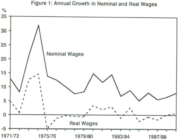
In 1983, an incomes policy (the Accord) was agreed to between the newly elected government and the Australian Council of Trade Unions. The Accord was part of the government's attempt to reduce the growth of nominal wages relative to productivity growth, thereby boosting employment. Figure 1 compares the growth in nominal wages over the 1970s and the 1980s. As is evident from that figure, nominal wage growth on average was much lower in the 1980s, especially from 1984, the year after the Accord was signed. Of more importance, especially for employment growth, was the behaviour of real wage growth which was considerably lower during the 1980s than the 1970s; in particular, a period of negative growth in real wages began in 1985. These issues are more fully discussed in Chapman (1990). As far as the monetary authorities were concerned, this lowering of nominal wage growth exerted downward cost pressure on the rate of inflation. The idea that cost variables have been seen as important proximate determinants of the rate of inflation (more so than monetary growth) is discussed in Carmichael (1990). As a result, the RBA appeared to believe that these developments would take care of inflation.
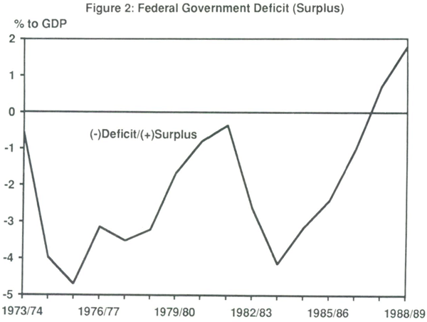
An important development during the 1980s was in the area of fiscal policy. Figure 2 shows the ratio of the federal government deficit to gross domestic product (GDP). This ratio, which was quite high during the 1970s and 1980s, fell dramatically as the government attempted a contraction in government spending as part of its long-term restructuring plan for the Australian economy. By 1987, the federal government deficit had become a surplus (see Edey and Britten-Jones (1990) for a more complete discussion). Whilst fiscal and monetary policies were not entirely independent (especially given the operating procedures of monetary policy prior to 1983), this had a major effect on the framework on which monetary policy had to be conducted. It meant that with fiscal policy largely being determined by a long-term strategy, only monetary policy was left to be any sort of counter-cyclical tool.
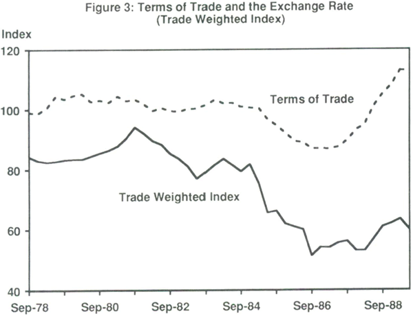
The third important economic development in the 1980s was the behaviour of the terms of trade, that is, the ratio of the price of exported goods to the price of imported goods. As Figure 3 displays, there were two falls in the terms of trade during the decade: one at the start of the decade (early 1980 until early 1982), and another fall beginning in late 1984 until the end of 1986. This behaviour of the terms of trade was primarily due to variations in the price of agricultural commodities, on which Australian exports largely depend. The direct effect of changes in the terms of trade is upon income, via the income of exporters. It also affects the exchange rate (also shown in Figure 3), which also has implications for monetary policy. As shown in Figure 3, the behaviour of the exchange rate (the price of Australian dollars in terms of foreign currency) paralleled that of the terms of trade over the post 1983 period.
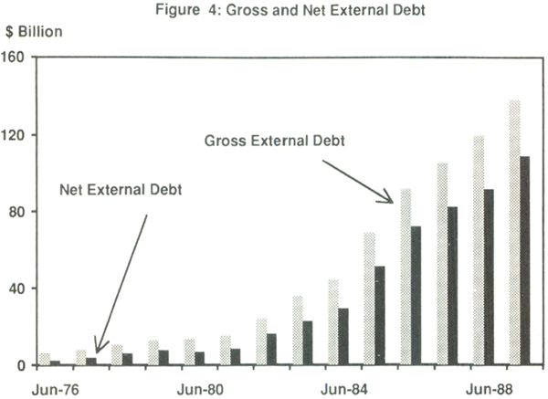
A fourth development, not unrelated to the conduct of monetary policy or the behaviour of the terms of trade, has been a rise in Australia's net external indebtedness, displayed in Figure 4. In part this is also related to changes in the regulation of financial markets. This increase in external indebtedness constrained demand management and thus monetary policy, especially in the latter half of the decade, and is an issue of current debate.
3. Monetary Policy
(a) The goals of monetary policy prior to deregulation
The theory of monetary policy, and its practice, were in transition during the 1970s. The dominant school of thought in 1970 had a Keynesian flavour. This was that monetary (and fiscal) policy should be used for fine-tuning in order to stabilize economic activity and reduce the amplitude of the business cycle. The attempt had been to target a real variable, such as real income or the unemployment rate, and to use expansionary monetary policy (an increase in the money stock or a reduction in interest rates) when unemployment rose above some normal level (later to be called “the natural rate”). This exploited a Phillips curve trade-off[1] between lower unemployment and a higher inflation. The arguments against this were given by Milton Friedman (1968) largely on two counts. First, Friedman argued that the lags from changes in the money supply (seen as directly controlled by the central bank) to economic activity were long and variable, so that fine-tuning was difficult and might make the business cycle worse. Second, attempts to permanently lower the unemployment rate would lead to accelerating rates of inflation as expectations of higher inflation were built into wage contracts.
The simultaneous increase in inflation and unemployment during the first half of the 1970s converted a number of economists to Friedman's position. Real variables, such as unemployment and the growth of real output were seen as being inappropriate targets. Instead this view argued that monetary policy should focus on the control of a nominal variable, in particular, the price level or its rate of change. A strong form of this view was that the central bank should pre-announce growth rates for the money stock and adjust policy to achieve them, independently of the state of the business cycle. This view was further strengthened by the work of Robert Lucas (1972) who argued that if a policy of fine-tuning is expected, it will have no influence on the business cycle. In this situation, expansionary monetary policy (if anticipated) will result almost immediately in a higher rate of inflation and little change in real variables (lags are short and certain). This was a return to the classical monetary prescription. This argument probably convinced a large enough audience that the link from money to prices was swift enough that announcements of contraction in the monetary growth rates would result in fairly quick deflation. In other words, targeting the growth rate of the money supply (monetary targeting) was the appropriate monetary policy. This not only represented a change from counter-cyclical policy, but a change in focus: from targeting a real variable to targeting a nominal variable.
Whilst academic economists were divided about appropriate policy (see for example Modigliani (1977)), central bankers moved towards the Friedman position. Beginning in 1975, many central banks moved towards monetary targeting, generally selecting a monetary aggregate whose growth rate was to stay within certain bounds. In these experiments, one of three alternative definitions of the money stock was used: the monetary base (MO) which consisted of the liabilities of the central bank (generally the stock of currency plus the reserves of the banks); M1 which (in Australia) consisted of currency plus the stock of current deposits at trading banks; or M3, which consisted of currency plus the total deposits of all trading and savings banks. From the banks' balance sheet identities, M3 can be alternatively defined as approximately M0 plus the total lending of the trading and savings banks. The RBA selected M3 but appeared to be less doctrinaire than the central banks of other similar countries such as Canada. The first discussion of targets occurs in the RBA Annual Report of 1979, which mentions that the RBA did not expect to stick to these targets rigidly. The RBA has stressed that these “targets” were seen at the time as conditional projections (Grenville (1989)) for reasons discussed below.
Thus the change in the stance of policy coming into the 1980s was a pre-occupation with inflation rather than fluctuations in real variables. This reflected two views. First, it was thought that monetary policy could do more to reduce inflation than it could to smooth out fluctuations in real variables. Second, policy makers perceived that inflation was seen by the public as a more important problem than fluctuations of real variables over the business cycle.
On the latter point, few tests to discover the public's aggregate preferences have been attempted, certainly for Australia. It is interesting to note that in a recent study in the U.S., Garman and Richards (1989) estimate preferences for inflation and output variability using Presidential popularity polls and other variables. They find the public's preferential rate of inflation, ceteris paribus, to be 0.21 per cent, some 4.72 percentage points below the actual average outcome over 1961–1986. Of course, the higher rate of inflation may have been accompanied by lower output variance than would otherwise have occurred. For the average person to be indifferent between the actual outcome (inflation, output variance) to one with the preferred inflation rate, the output variance accompanying the 0.21 per cent and preferred inflation rate would have to have been twice the actual output variance. Garman and Richards claim that Modigliani's (1977) calculations suggest that discretionary policy did lower the output variance by about one-half. Thus if counter-cyclical policy did contribute to a higher-than-preferred inflation rate, it neither raised nor lowered welfare, a sobering thought for all policy makers.
(b) The operation of monetary policy prior to deregulation
There were three sets of regulations that the RBA used during the 1970s in the operation of monetary policy. The first was interest rate restrictions on deposits and loans of the trading and savings banks, restrictions that stifled each bank's ability to increase its deposit base. In addition, there were restrictions on the terms of fixed deposits. Second, the RBA often suggested quantitative lending guidelines for banks, to restrict the creation of bank credit. Third, the RBA used portfolio restrictions, such as the Statutory Reserve Deposit (SRD) ratio, to vary the liquidity position of the banks. There were two other considerations in the operation of monetary policy. The first was that, while most of the developed world operated on a flexible exchange rate system, Australia operated a crawling-peg system which, for monetary management purposes, was more like a fixed exchange rate. The other consideration was the way in which government debt was sold; an interest rate was established and the demand for paper by the private non-bank sector determined how much was taken up by the banking system.
The impact of these last two considerations meant that the RBA was unable to hold much sway over the extent to which movements in the government's accounts and the balance of payments affected the growth of M3. This is reflected in the official RBA presentation of its statistical tables in which changes in the money stock (M3) result from changes in foreign currency, changes in the public sector borrowing requirement (less private purchases of government debt) – both of which are outside its control – and changes in bank lending – which it can influence. Policy tools were therefore mostly directed towards bank lending. But the fact that the RBA saw much of the money stock as outside its control is presumably why it had to regard monetary targets as conditional projections.
The RBA saw its role mainly as one of influencing lending, and of smoothing liquidity over the seasonal patterns of the year. A look at the RBA Annual Reports confirms that there is little discussion of the RBA's contribution to policy outside of these areas, and comments about slowing the rate of monetary growth do not appear until 1979/80. Because of the institutional arrangements, open market operations (OMO), in which government bonds were bought from or sold to the public, were limited in scope. In addition, the RBA was limited in its ability to reverse the effects of changes in the monetary base. Active use of the SRD ratio would end up denying reserves to the banking system which would cause the kind of liquidity crises that the RBA was charged with avoiding.
(c) Financial innovations and deregulations
The regulations imposed by the monetary authorities acted to restrict the flow of credit, often forcing banks to ration. Interest rate restrictions also reduced competition between the banks, and reduced the banks' ability to compete with the non-bank financial intermediaries (NBFIs) who were not restricted. There were two reactions. One was a theoretical debate about the relevance of regulations; the other was a policy reaction to the innovations that the regulations produced.
From a microeconomic viewpoint, several economists saw these interventions as welfare-reducing and unnecessary. This prompted a call among academic economists, of which Porter's (1979) survey is an example, for an end to each type of regulation. Black (1970) began the “free banking debate” by arguing for a laissez-faire approach to banking free of distortions and intervention. There were two particular aspects to this: whether monetary authorities should restrict intermediation between private individuals, and whether the government should have a monopoly on the issue of currency. Leaving the second issue aside, Fama (1980, 1983) claimed that restrictions on credit creation were unnecessary, since control of an aggregate such as the monetary base (which largely consists of currency) was sufficient to tie down the price level in theoretical models (that is, nothing stops us defining the money supply as M0). Sargent and Wallace (1982) then constructed an example to show that restrictions on private intermediation are sub-optimal (according to the Pareto criterion) in a general equilibrium model. A survey of this debate is given in MacDonald and Milbourne (1990). Harper (1984, 1988) discusses the related question of how a price level might be defined in a world in which there were no regulations and no demand for currency (taking the Fama argument one step further). In this case, there would be no price level of goods in terms of currency, but since currency wasn't being used, nobody would care: the price level could be set in terms of one of the commodities.
The deregulations of the Australian financial markets (discussed below) had little to do with the academic debate above, but were more intended for practical considerations. To a large extent, these deregulations were the response to innovations by the banks to the higher rates of inflation and interest rates in the 1970s. The regulations outlined above had been useful for banks because they helped keep down the cost of obtaining funds from the public. However, with the general rise in interest rates, the interest rate ceilings on banks became binding. This caused a switch of deposits by the public to the NBFIs who were not subject to these interest rate (and other) restrictions and who could offer higher deposit rates. The loss of market share prompted the banks both to exert pressure for changes in the financial system directly, and to search for innovations that would get around the restrictions. As a result, banks began to engage in off-balance-sheet business in which they would, for example, act as a loan broker between two parties, receiving a commission. This was not subject to interest rate restrictions, and since it never appeared on the books, it did not require the holding of a proportion of the transaction as SRDs. In addition, loans could be routed through overseas subsidiaries to reduce taxation liability.
The realization that banks were innovatively circumventing most of the legislation, and that the remaining regulations were unfairly disadvantaging the banks, prompted a re-think of monetary policy operation. The choice was between throwing the regulatory net wider to cover the NBFIs and other bank operations,[2] or removing the direct controls. In 1979, the Campbell Committee was formed to evaluate the Australian financial system and recommend policy changes. This committee of inquiry received voluminous submissions (Australian Financial System Inquiry (1982)) and recommended major deregulation of the financial system and policies to promote competition in banking in its findings, submitted in 1981. With the change of government in 1983, the Martin Review Group was formed to determine which of these recommendations were within the philosophy of the Australian Labor Party. This report supported the call for deregulation.
A chronology of the major deregulations is contained in Table 1. More detailed lists of changes to the financial system are contained in Battellino and McMillan (1989) and the RBA Bulletins, and financial innovation bibliographies are given by Moses (1983) and Boulton and Tease (1984). The deregulations can be put into groups corresponding to those given above. Interest rate restrictions on bank deposits were removed in December 1980 before the release of the Campbell findings, and regulations on the terms of fixed deposits and certificates of deposit were relaxed in August 1981 and March 1982, and abolished in August 1984. This meant that following August 1984, banks could actively enter the short-term money market (STMM) and compete for funds.
| 1980 | |
|---|---|
| December: | Interest rate ceilings on all trading bank and savings bank deposits were removed. |
| 1981 | |
| August: | Minimum term on certificates of deposit was reduced to 30 days. |
| 1982 | |
| March: | Minimum term on trading bank fixed deposits (> $50,000) reduced from 30 to 14 days, and for fixed deposits (< $50,000) from 3 months to 30 days. |
| Minimum term for certificates of deposit reduced to 14 days. | |
| The requirement of one month's notice of withdrawal on savings bank investment accounts was removed. | |
| June: | The end of quantitative lending guidance. |
| 1982 | |
| August: | Savings bank asset requirements reduced to 94 per cent, and prescribed asset ratios relaxed. |
| 1983 | |
| December: | Australian dollar floated and most foreign exchange controls removed. |
| 1984 | |
| August: | All remaining controls on bank deposits removed. |
| Savings banks permitted to offer chequeing facilities. | |
| 1985 | |
| February: | 16 foreign banks invited to take up banking licences. |
| April: | Remaining ceilings on bank interest rates removed, except those on owner-occupied housing loans under $100,000. |
| May: | The Prime Assets Ratio (PAR) replaced the LGS convention. |
| September: | The first foreign bank began trading. |
| 1986 | |
| April: | Interest rate ceiling on new housing loans removed. |
| 1987 | |
| April: | Savings bank reserve asset ratio reduced to 13 per cent. |
| 1988 | |
| September: | SRD ratio reduced to zero (previously had been 7 per cent for trading banks), and those funds transferred to “non-callable deposits”, with those funds in excess of 1 per cent of liabilities to be gradually returned to banks. |
| Free tranche for savings banks increased from 6 per cent to 40 per cent, as an interim step towards removing the distinction between savings banks and trading banks. | |
| PAR reduced from 12 per cent to 10 per cent. PAR to replace existing savings bank regulations. | |
| Source: Battellino and McMillan (1989) and Reserve Bank of Australia Bulletins | |
Quantitative lending guidelines were abolished in June 1982. Portfolio restrictions on trading and savings banks were relaxed sequentially in August 1982, May 1985 and April 1987, and the reduction of the SRD requirement began in September 1988, when it was replaced by a 1 per cent non-callable deposit. The two other obstacles to the operation of monetary policy were also removed. The Australian dollar was floated in December 1983. In addition, the system for selling government debt was changed, with the government and/or the RBA establishing the amount of bonds to be sold to the private sector, with the price determined by the market.[3] Finally, the Treasurer invited applications from foreign banks for trading bank licences in Australia to promote competition, and September 1985 saw the first of 15 foreign banks begin operations.
The main consequences of these changes were threefold. First, monetary policy would no longer operate with direct quantitative guidelines. Instead, monetary policy could only operate via affecting asset prices (or equivalently, interest rates). Secondly, it gave the RBA control over the monetary base,[4] since changes arising from the government budget deficit, private take-up of government debt, or changes in the current account would not translate into changes in the monetary base unless the RBA so desired. Third, it meant that substitutions between assets due to the deregulations, and further innovations in the payments mechanism (which continued throughout the decade) would make the monetary aggregates very difficult to interpret.
(d) Monetary policy and the behaviour of monetary aggregates
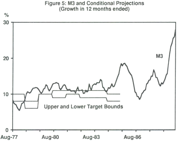
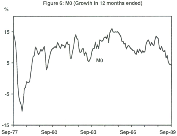
Australia entered the 1980s with the Treasurer issuing targets or conditional projections for M3. As Davis (1988) points out, after 1978 actual growth exceeded the projections almost every year, as shown in Figure 5. The RBA Annual Reports of 1979–1982 contain a list of the factors that led to excessive growth of M3 over this period, along with an annual promise that steps would be taken to slow the growth of money and credit. Prior to 1984, the RBA attributed the unexpected growth to large government budget deficits for which the private sector did not take up the corresponding bond issue. Also mentioned were current account deficits. These factors should also affect the monetary base; however, while these factors may have been important for day-to-day changes, Figure 6 shows that the 12-month growth rate of the monetary base during 1980–83 was probably below that of other periods. Of more importance appears to have been the relative growth of credit issued by the banks, which was under the more direct control of the RBA. Thus the failure to attain M3 targets was due more to the failure to restrict credit than M0, probably due to inflexibility of interest rates.
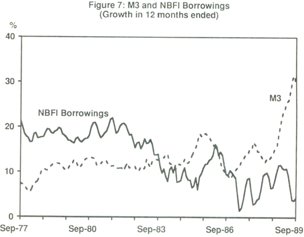
The relationship between monetary aggregates changed frequently during the decade. Figure 7 shows the 12 month-ended growth rate of M3, and the corresponding growth rate for borrowings from the public of NBFIs (i.e. deposits of the public at NBFIs). The higher growth rates for NBFIs continued until 1983 as restrictions on the banks were sequentially removed. During 1984–86, M3 grew more rapidly as banks were able to compete actively for funds. In particular, access to the STMM was responsible. Only a small part of this relative bank expansion was due to some NBFIs converting to banks or from the entry of new banks (Hogan (1989)). The period 1983–85 was referred to as the period of “re-intermediation”. The RBA argued that M3 would be a misleading indicator of monetary policy over this period. Thus they saw themselves in a difficult situation: at the precise time when deregulation had given them the tools for better control of the money stock, the chosen indicator became an unreliable guide to policy (RBA (1987)).
The RBA looked at broader aggregates to net out the effects of deregulation on M3. Two new monetary aggregates were created. Broad money (BM) added to M3 the borrowings from the public of the NBFIs. Also, attention was given to an even-broader financial aggregate, credit, defined as loans and advances by all financial intermediaries plus bank bill finance. This latter aggregate was intended to capture a larger proportion of total credit in the hope that it bore a stronger relationship to income. The RBA abandoned M3 targeting in January 1985, and replaced it with a “checklist” approach. In this approach, a variety of indicators would be considered including the rate of inflation, the exchange rate, interest rates, the balance of payments, the state of the economy and monetary aggregates (Johnston (1985)). The evidence (discussed below) seems to indicate that the exchange rate became the main focus of policy for at least the first twelve months (and probably more) of the “checklist”. The RBA has not referred to this “checklist” in recent years.
The behaviour of M3 over the last half of the decade was due to innovations by the banking system and further deregulation. After 1986, the growth of M3 fell because of a shift by the banks to off-balance-sheet business. With the reduction in the SRD ratio in September 1988, banks rearranged the liabilities side of their balance sheets, so that M3 surged while this adjustment was occurring.[5] As Figure 5 shows, the behaviour of M3 is heavily dominated by the innovations and deregulations of the decade.
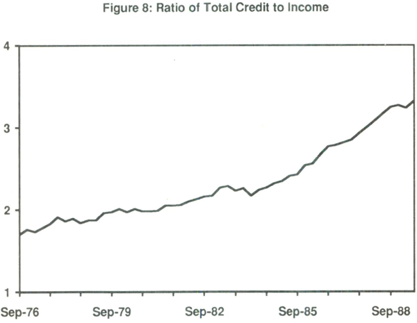
The unreliability of M3 was matched by the behaviour of the broader aggregates. Figure 8 shows the ratio of credit to nominal income. This ratio is the inverse of velocity; it shows a marked increase in the later half of the decade even when most of the deregulations had been completed. This unexplained increase in credit has been addressed by Macfarlane (1989a). Macfarlane argues that the high demand for credit may have been thwarted in the early 1980s by regulations that induced the banks to ration the quantity of credit. This is not entirely consistent with the timing of the change. A more likely reason would appear to be the distortions caused by the interaction of tax system and inflation. Full deductibility of nominal interest payments confers on borrowers a major tax advantage of debt over equity, since it reduces the after-tax real cost in inflationary times. Debt, intermediated via the financial system, raises broader aggregates including M3 whereas equity does not. As Macfarlane points out, bank lending rose by 18.8 per cent per year in the latter half of the decade, whereas deposits increased by only 12.8 per cent. The difference was made up by other forms of bank borrowings, especially overseas borrowing.[6] The rise of debt relative to equity confirms this trend. This raises the point that tax changes, such as imputation of dividends, will have a dramatic effect on the debt-equity choice, which has a direct effect on broad monetary aggregates. Figure 8 illustrates that even when the deregulations were mostly completed, changes originating outside of the financial sector had a dramatic impact on the relationship of financial aggregates to income.
(e) The debate about the conduct of monetary policy in Australia
There was relatively little debate in Australia about the philosophy behind Reserve Bank policy during the 1980s. In the United States and Canada, for example, attempts to adhere rigidly to narrow monetary targets polarised economists and produced a lively debate about the philosophy of monetary policy.[7] I put this down to the fact that the attitude of the RBA was less doctrinaire than that of the other central banks,[8] and the fact that until 1983 there was little scope for the RBA to achieve those projections because of the pegged exchange rate and RBA operating procedures. Thus, monetary policy was difficult to debate because the money stock was endogenous. Many have argued (see below) that even after 1983 the money stock was endogenous given the operating procedures of the RBA. In addition, financial innovation and deregulation has made targeting difficult, and so appropriate policy has been less clear. Indeed, the lack of information in M3 has made it difficult to classify monetary policy as tight or easy. One measure often used in this regard is the yield curve. Tight monetary policy raises interest rates at the short-maturity end of the asset yield curve. If this policy is expected to be relatively temporary, then short-term rates rise above long-term rates giving an inverted yield curve. The same situation occurs if current tight monetary policy is expected to lower future inflation rates and thus lower the inflation premium of future nominal interest rates (on which current long-term interest rates are presumably based).
The objectives of RBA policy changed many times during the decade, with a consequent lack of consistency. Whilst the RBA Annual Reports indicate that inflation was an initial objective, the RBA interpreted the Accord as taking care of this, and directed policy towards maintaining economic activity during 1984. This view seemed to change abruptly in 1985 as concern for the rising current account deficit and the instability in foreign exchange markets arose. Concern about the stock market crash of October 1987 caused the RBA and other central banks to believe that growth in demand would reduce inflation without a monetary policy tightening. By late 1988 concern had switched back to inflation and external imbalance. This lack of consistency in policy is discussed in Stemp and Murphy (1990).
In discussing monetary policy, it is useful to consider three time periods:
- the very short run (or day-to-day) behaviour in which the RBA might attempt to smooth interest rates or exchange rates (by removing “noise” and thus reducing the variance of the variable in question);
- the short run, in which the RBA might attempt stabilisation policy; and
- the long run, in which the RBA attempts to control the rate of inflation.
Unfortunately, economic theory does not say anything about how long the short and long runs are. Undoubtedly the introduction of rational expectations into macroeconomic models convinced many that the short run was very short. This prompted the opinion that if monetary targeting was designed to reduce inflation, it should do so quickly. Many economists, such as Milton Friedman, saw monetary targeting as a short-run as well as long-run policy. According to Grenville (1989), the RBA saw targeting as only a long-run program of winding inflation down over time. That is, the announcement of monetary targets was intended to anchor expectations over the longer term. The issue is whether commitment to a long-run average rate of monetary growth allows the RBA to respond to short-run shocks without compromising longer term objectives. Certainly, a reading of the RBA Annual Reports indicates that the RBA believes that the answer to that question is “yes”. Stemp and Murphy (1990) argue that the answer is “no”: such short-term changes make long-term expectations-formation impossible.
The issues debated over each time period seem to be the following:
(i) The very short run
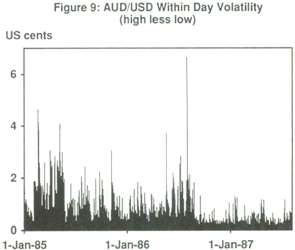
The debate has been whether the RBA should smooth out daily fluctuations, and in what variable. For example, Shields (1988) and Marsden and Jones (1988) maintain that beginning in January 1986, RBA policy became a de facto one of smoothing the exchange market (that is, returning to something like a pegged exchange rate). McTaggart and Rogers (1989) (hereafter MR) claim that there have been more interventions in the exchange market in the 1980s than in the 1960s, as measured by the percentage changes in foreign currency holdings of the RBA. Both Shields and Marsden and Jones maintain that since 1986, there has been increased interest rate volatility and less exchange rate volatility. Figure 9 (reproduced from Marsden and Jones) shows that within-day volatility of the exchange rate halved in 1986. Shields similarly shows an increase in the volatility of interest rates.
(ii) The short run
The general perception in the 1980s of the role of monetary policy in the short run is that it has been the first-in-line policy tool for counter-cyclical policy (e.g., Parker (1989)). In part this reflects a desire on the part of the Commonwealth government to reduce substantially the government budget deficit, and a commitment to that goal essentially ruled out the use of fiscal policy as a significant income stabilisation tool. Thus, monetary policy had to act alone as a short-term counter-cyclical tool. This may explain the fixation with short-term disturbances that is a feature of the RBA Annual Reports.
A related question is whether the RBA attempted to prevent some of the exchange rate depreciation in 1985/86. This would be plausible only insofar as the RBA believed that the dramatic changes in the exchange rate were temporary, or that the exchange rate was overshooting its equilibrium value because of excessive speculation. Indeed the behaviour of the exchange rate (Figure 3) indicates that, had the RBA believed this, they would have been correct. The government's reason for avoiding a dramatic depreciation was to prevent the inflationary effect on the price level and the resulting effect upon the Accord. By raising the Australian prices of imported goods, a depreciation flows through to the Consumer Price Index (CPI). This would have put the Accord under considerable pressure. Since the Accord was a major part of the economic policy of both restraining inflation and increasing Australia's ability to compete via a reduction in unit labour costs, such a breakdown would have short-term and long-term consequences. Richards and Stevens (1987) survey empirical estimates of the elasticity of the price level with respect to the exchange rate. These estimates range from 0.23 to 0.36. They estimate that the depreciation added 12 percentage points to inflation over the two years.
A related issue is the response of the RBA to changes in the terms of trade. Figure 10 shows the growth rate of the monetary base against the terms of trade. MR criticise RBA policy as it relates to the terms of trade deterioration in 1985/86. The RBA insisted on a firm monetary policy (a reduction in M0 growth) to combat any inflation which would follow from the resulting exchange rate depreciation. This is again in line with the broader government policy objective involving the Accord. MR claim that the response of monetary policy should have been expansionary to alleviate the fall in income. Which view one accepts depends upon the relative weights attached to avoiding inflation relative to avoiding output loss. MR further raise the point that, in general, monetary policy has been pro-cyclical with respect to the terms of trade. This is true of the 1985/86 period. This may follow because the operating procedures of the RBA, and in particular the attempt to hold the exchange rate and/or the interest rate, meant that the money stock became endogenous; in particular, falls in income would be reflected in a reduction in the demand for money.
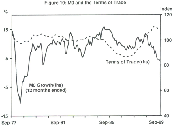
Apart from the 1985/86 period, it is difficult to support the MR hypothesis, as Figure 10 shows. There seems to be little correlation between M0 growth and the terms of trade either prior to 1985 or after 1986. Of course, within the broader issue of economic policy, Poole (1970) and subsequent analysts have shown that monetary policy should never be used to react to real disturbances such as terms of trade changes. In the simplest models, use of fiscal policy minimizes both interest rate and output fluctuations in response to a real shock, and monetary policy does likewise for a monetary shock. This is insofar as these policies work quickly to restore equilibrium (for which there is little empirical support) and this issue is dealt with in more detail below in Section 4(b).
(iii) The long run
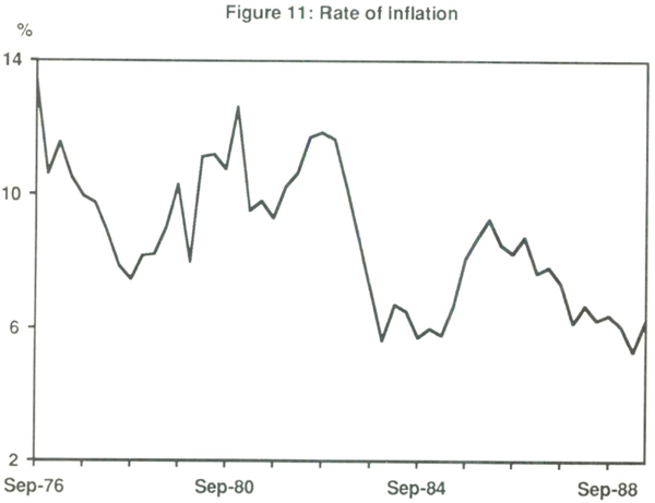
MR have also been critical of long-run RBA policy, claiming that the RBA should target the monetary base (MO). They make the point that the RBA could easily change operating procedures so that M0 would be directly under their control. Currently, the RBA extends lender-of-last-resort facilities to the authorized dealers. This means that M0 is endogenous since authorized dealers can always borrow at the (fixed) re-discount rate if market interest rates rise. MR argue that the RBA should have set a fixed target path for M0, and varied the re-discount rate to achieve it. The implication is that inflation would have been lower under commitment to a monetary base target. As Figure 11 shows, inflation has been lower during the 1980s than during the 1970s, except for the 1985/86 period when the exchange rate depreciation which accompanied the terms of trade deterioration clearly affected the inflation rate. Whether inflation would have been even lower with M0 targeting is a counter-factual question. As Carmichael (1990) reports, inflation in Australia appears to be more a function of non-monetary factors than monetary ones. That is also one of the implications if one compares the inflation decline in Figure 11 with the behaviour of monetary aggregates. Nevertheless, it may be that failure to state an anti-inflationary position conditioned those variables that do appear to influence inflation.
4. Empirical Macro-economic relationships
Macroeconomic theory is generally uninformative about the dynamic structure of relationships between variables. However, the conduct of monetary policy relies on those empirical relationships. To understand which relationships are important, it is worthwhile to consider the transmission mechanism of monetary policy.
(a) The transmission mechanism
The standard transmission mechanism of monetary policy works via its effects upon interest rates. An open market operation (OMO) is a swap of government securities for money and so has little effect upon wealth. Table 2 presents the standard “textbook” transmission mechanism of an OMO.
| → |
aggregate demand | → |
output, labour market |
→ |
prices |
|||||
| open market operations |
→ | cash rate | → |
other interest rates |
||||||
| → | exchange rate | → | output, prices | |||||||
| → | intermediaries' balance sheets |
→ | monetary aggregates |
|||||||
The two main issues inherent in the transmission mechanism are:
- what is the lag between monetary policy and each of the variables? and
- what, if any, is the relationship between the effect of changes in interest rates on economic activity (the top two lines of Table 2) and the effect upon monetary aggregates (the bottom line of Table 2)?[9]
If the change in monetary policy were anticipated, and all prices were completely flexible, Lucas (1972) has argued that there would be no real effects, and that prices would immediately rise (that is, the transmission mechanism would be very quick). If the change were unanticipated, or if there were short-term nominal rigidities, then we must consider each possible lag. (Empirical evidence on each lag is given in the next section).
An OMO affects the cash position of the authorized dealers, which in turn affects the cash rate (the interest rate which clears the cash market). This occurs quite quickly. From here, however, the time lags are unclear. It depends upon whether the change in RBA policy which produced the OMO is believed to be permanent. If not, even short-term market rates will be unlikely to change. In this case, the cash rate would have to continue at its new level for some time in order to induce a change in other bank interest rates.
The second lag is that between changes in interest rates and changes in aggregate demand.[10] Investment is typically regarded as the most interest-sensitive component of aggregate demand. The relevant interest rate is the real (after-tax) interest rate. Since investment projects have a relatively long average payback period, it is the long real rate which is probably more appropriate. However it is not clear how reliably, and over what time periods, changes in short nominal rates can affect long real rates. Even so, most investment plans take some time to formulate and/or implement; they add to aggregate demand only when the new investment has been ordered.
The third lag is between changes in aggregate demand and changes in output. An initial reaction by firms to changes in demand is to accumulate or decumulate inventories and leave production unchanged. This does not affect GDP since on the expenditure side of the accounts, changes in planned expenditure and inventory accumulation offset each other. Only if firms believe that the change in demand is more permanent do they alter production rates and it may take some time before they are convinced that the change is permanent. The change in demand may induce some price changes as well although once again these effects are likely to be gradual.
The change in output will affect the demand for labour. Given the relatively rigid short-run nominal wage outcomes in Australia which are a feature of the periodic national bargaining system, this will impact mostly on employment in the short run.[11] Only over a longer period will a change in wages occur, which then gives an additional, longer-lagged effect upon the price level.
A second link in the transmission of monetary policy is via the exchange rate, and has only recently been stressed (e.g., Blundell-Wignall and Gregory (1989)). Changes in domestic interest rates will cause a change in the interest differential between domestic and overseas rates. With a high degree of capital mobility, this results in changes in capital flows. The expectation of these flows is sufficient for the foreign exchange market to anticipate a change in the exchange rate; [12] this brings an almost immediate change in the current exchange rate as dealers attempt to take advantage of the new information.[13] The change in the exchange rate has a number of effects. For exposition, consider an exchange rate depreciation.
The first effect is that imports become more expensive in Australian dollars, which raises the general price level. The second effect is on output. The depreciation causes a relative price fall for domestically-produced non-tradable goods and services with respect to tradable (imported) goods. If the change in the exchange rate is considered permanent, this should increase demand for non-tradable goods. Since most of Australia's exports are in agricultural and mineral commodities whose prices are generally set in terms of a foreign currency, the income of exporters should rise in Australian dollars, thus also adding to demand. The first output effect, a net change towards domestically-produced goods, is likely to occur with a considerable lag because these substitutions between domestic goods for imports are probably not made quickly. The second possible effect on output, the direct income effect to most exporters, may not affect output immediately if these exporters treat the income as transitory and behave according to the permanent-income hypothesis. Finally, any increases in demand will cause an additional inflationary effect upon the prices of non-tradable goods. Of course, this effect may occur with a considerable lag.
This part in the transmission channel has become more important since the floating of the Australian dollar. It is also likely to be important if aggregate demand is relatively insensitive to the interest rate, as would appear to be the case below, and from Edey and Britten-Jones (1990). Blundell-Wignall and Gregory (1989) believe that this channel is now the most important for Australia.
Changes in interest rates will also impact upon the balance sheets of financial intermediaries. Changes in the nominal interest rates on bonds and similar assets will cause a portfolio shift to or from bank deposits.[14] This immediately affects the monetary aggregates. It is likely that these changes would precede those in the goods markets. Consequently it might be thought that changes in money growth would (perhaps systematically) precede changes in output and prices. This however ignores an important feedback between each of the variables which dramatically complicates empirical investigation of the lags involved in monetary policy. Since this is important for the next section, it is worthwhile considering in detail.
Monetary aggregates, output, and prices may change for reasons other than changes in monetary policy. Shocks in exogenous variables such as export demand, the terms of trade, floods or drought, and financial innovation all affect each of the variables of focus with different timing, and therefore set up feedback relationships. For example, an exogenous fall in export demand lowers income. This leads to a reduction in the demand for money which, given the short-run operating procedures of most central banks, implies a reduction in the money stock. If money lags income, then this is the reverse of the timing suggested above. Similarly, agricultural harvest failures lower income but raise the general price level, giving the reverse correlation from that of the standard Phillips curve inherent in the above discussion. Moreover, the price rise increases the demand for money, so that exogenous changes in the price level may cause price changes to precede changes in the money stock.
It follows from the above discussion that simple examination of the average lag between two variables is unlikely to uncover timing relationships that are sufficiently reliable to be used in economic policy. This is because the sample from which the “evidence” is gathered is likely to have experienced a predominance of one type of shock relative to another. This evidence is useless if the current period is facing different types of shocks. One approach might be to use a large econometric model which identifies all possible shocks, and thus nets them out of the temporal relationships between monetary policy aggregates and economic activity. This is a difficult task. In the first place, there have been many regime shifts, each of which will change the nature of the lags. In the pre-deregulation period, a restrictive monetary policy could operate via direct quantitative restrictions which might directly curtail spending and thus substantially reduce the first two lags. Moreover, the relationship between aggregate demand and interest rates will differ when quantity rationing is prevalent, from that relationship operating in an unrestricted setting. Currently, therefore, we would only possess relevant data from 1984 onwards, or less than 30 quarterly observations, which is insufficient to establish empirical relationships with any confidence.
In particular, the relationship between money and prices is tenuous, especially over the short and medium term. This reflects the fact that the transmission mechanism affects each via a different set of lags, as evident in Table 2. As we show below, it is very difficult to establish a reliable link between money and prices. Reasons for this are also advanced below.
(b) Empirical evidence on the transmission mechanism
The econometric difficulties discussed above are reflected in wide disagreement about the empirical relationships between variables, especially their timing. In this section we discuss the conventional wisdom about these relationships, as reflected in recent writings, in the order discussed above.
Marsden, Healey and Doyle (1989) have argued that a change in the cash rate typically affects bank bill rates almost immediately. They guess that these changes affect the prime overdraft rate with a 1 to 3 week lag (presumably if expected to be permanent), with 3 to 4 week lag to changes in the fixed deposit rate. They argue that these then filter through to mortgage rates. If so, this indicates that the lag from monetary policy to relevant interest rates is of the order of two months or less.
The lags from interest rates to economic activity are more problematic. Oster (1988) surveys a wide variety of models, from econometric models to simple reduced-form equations. The lag from changes in monetary policy to income varies from 9 months to 18 months, with a further lag to prices. This variance almost certainly reflects the econometric problems discussed above. Davis and Lewis (1978, 1980) claim that the lag from money to prices up until the 1970s was approximately 12 months. If correct, it would imply that lags have been lengthening during the 1980s, since those studies reported in Oster include 1980s data. On the other hand, work at the Research Department of the RBA (discussed below) casts doubt on these relationships.
The best illustration of why opinion differs on the relationships is graphical. Figures 12 to 16 display some of the relationships between the key macroeconomic variables. Figure 12 displays the behaviour of the nominal and the real interest rate since the mid 1970s. The real interest rate is defined as the ex post rate, in order to avoid troubles of proxying for price expectations. The nominal interest rate is the 90 day bank bill rate. There are two important facts that come out of Figure 12. The first is that the behaviour of the real interest rate relative to the nominal rate was much different in the 1980s than it was in the 1970s. In the 1980s the nominal and real rates were much more closely aligned, and this reflected a much steadier and less variable rate of inflation. In the 1970s the ex post real rate was highly variable, being negative for a long period of time.
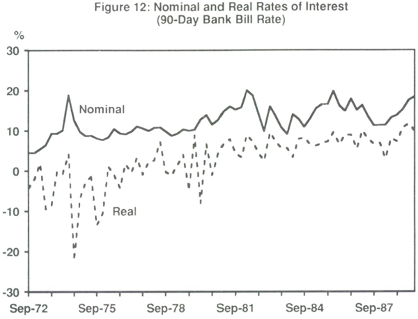
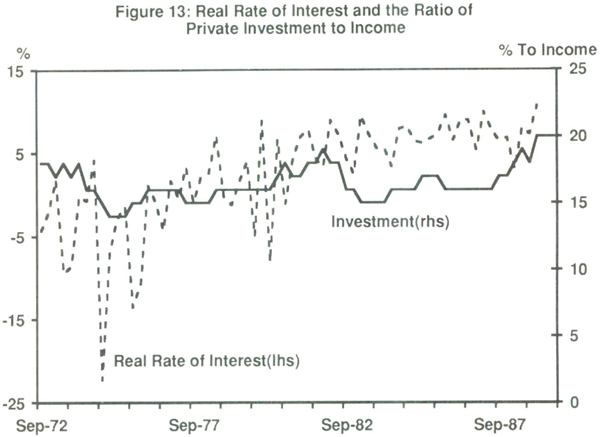
The second important fact is the average increase in the real interest rate over the period, particularly the steady increase in the real interest rate over the 1980s. According to the standard transmission mechanism, if the real interest rate is the main determinant of investment expenditure, then we would expect to see a negative relationship between investment and the real interest rate. Figure 13 shows the real interest rate (in percentage terms) against the private investment-to-income ratio.
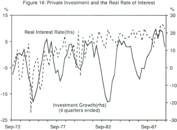
Whilst the investment-to-income ratio appears to be mean reverting, the real interest rate turns upwards over most of the sample period. In the language of econometrics, it is very difficult to see how these two variables would be co-integrated. Figure 14 presents the evidence slightly differently. It shows the real interest rate against the 4 month growth rate of real private investment. There are a number of features in this diagram worth mentioning. First of all, periods of increased growth in investment are not correlated with a lower real interest rate; in fact, periods of high investment tend to be correlated with higher real interest rates.[15] Secondly, as is also shown in Figure 13, investment has been relatively high in the second half of the decade despite the generally high real interest rate. This evidence is, of course, consistent with investment being largely determined by exogenous or demand-driven factors, and it may be that investment has driven the real interest rate rather than vice versa (see below). This would follow if periods of higher investment led to increased pressure on the demand for funds. Of course, in an open economy, this effect would be weaker. Evidence seems to suggest that the real interest rate in Australia has closely followed the U.S. real interest rate since 1983, although over time the Australian rate has been rising relative to the US rate.
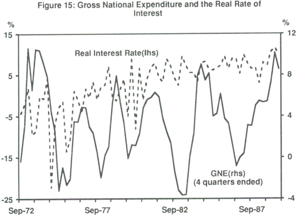
It may be that other components of aggregate expenditure are more interest sensitive, and therefore it is really the effect of interest rates on aggregate expenditure which is important. Figure 15 shows the real interest rate against the 4 quarter-ended percentage growth rates of real gross national expenditure. As that figure illustrates, there is virtually no relationship between the real rate of interest and the growth rate of expenditure in the 1980s. Of course, such graphical analysis does not really test whether at the margin real interest rates affect aggregate expenditure, or with what lag.
Research at the RBA has failed to find such relationships. Consider first the money-income relationship. Bullock, Morris and Stevens (1988) [BMS], Bullock, Stevens and Thorp (1988) [BST], and Stevens and Thorpe (1989) [ST], all show that for the 1980s, M3 and broader aggregates lag both nominal and real income, so that they are unsuitable as leading indicators of economic activity. This conclusion was made on the basis of graphical analysis (BMS); and Granger-Sims causality tests in levels (BST) and first differences (ST). In terms of the transmission mechanism, this is consistent with interest rates affecting monetary aggregates more slowly than they affect economic activity.
For narrower aggregates, the evidence is ambiguous. BMS claim that Ml leads final spending, although the data were heavily smoothed. ST find that M1 leads nominal GDP for the period 1978–1988, but the evidence does not support this proposition for private final spending.[16] The problem is that Ml is very difficult to control because of substitutions between current and non-current accounts and financial innovations in the payments mechanism. Thus the only monetary aggregate which leads activity (and thus helps predict it) is not easily controllable; those which are controllable follow rather than lead changes in activity. Also, Ml is clearly endogenous.
Little statistical research has been done on the monetary base. Sieper and Wells (1989) present graphical evidence that the growth rate of M0 less 4 per cent and lagged six quarters has a reasonable fit with the rate of inflation (as measured by the Consumer Price Index). Of course if one is free to choose the constant to subtract plus the lag, it is always likely that one can produce a reasonable graphical comparison. Home and Monadjemi (1985) find that M0 is the worst monetary aggregate as a predictor of real output. In a series of regressions they allow each monetary aggregate (with lags) to predict output separately. They find the best aggregate to be M3, followed by Ml, bank lending, and lastly the monetary base; on other grounds, bank lending is more stable than total indebtedness of the non-financial sector, which they subsequently dropped from their analysis. In particular, the last two were terrible predictors of output; bank lending had an R2 value of around 0.1 (when the equations were in levels!).
As would be expected from the figures discussed above, establishing an empirical relationship between interest rates and activity is difficult. BMS attempt to show a link between interest rates and economic activity. However, that study concentrated on nominal interest rates and the data were smoothed with a moving average procedure. BST show that statistical analysis on the original data is unable to discover any strong lead or lag relationship (causality) between interest rates and economic activity. Moreover, ST show that with differenced data the causality appears to run from nominal income to interest rates (which is the opposite of the standard transmission mechanism); if there is any feedback relationship in which interest rates affect income, it is very weak.
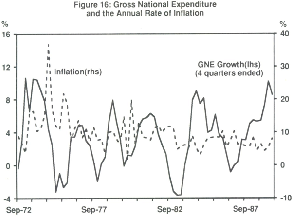
Figure 16 displays the relationship between the 4 quarter-ended growth rate in expenditure (GNE) with the 4 quarter-ended growth rate of the gross national expenditure deflator. That graph has two important features; the first is that inflation has been much less variable in the decade of the 1980s than in the 1970s. The second feature is that inflation has not come down to a level consistent with that of Australia's main trading partners (whose average inflation rate is about 5 per cent). A further important result that the graph seems to suggest is the lack of correlation between inflation and GNE growth. In fact, if one takes a crude measure of the correlation between the two, it is negative. This finding goes against standard Phillips curve literature in which GNE, or demand, is supposed to exert a positive effect upon the rate of inflation (or vice versa in the Lucas version). What seems to be true in Australia is that inflation is very weakly – if at all – related to output growth, and it has generally been a function of other variables such as wages growth, changes in terms of trade, and other cost factors. These issues are discussed more fully in Carmichael (1990). In fact, the negative correlation that is reflected in Figure 16 suggests supply-side shocks such as terms of trade and other shocks have been dominant. Adverse supply-side shocks tend to increase both the price level via costs, and to decrease output. Adverse productivity shocks have the same effect. Without full econometric evidence, a casual conclusion is that these effects have a much greater role to play in inflation than does output, and therefore one has to question part of the standard transmission mechanism of interest rates (and money) via income to prices.
(c) The stability of M3
A standard way of considering the empirical relationships between money and other variables involves the money demand function. If the effects of changes in monetary policy are to have predictable outcomes with predictable lags, the demand for money function must be reasonably stable. One finding of the 1970s was that these functions were not stable, and were very poor forecasters. A survey of these studies is contained in Davis and Lewis (1978) who point to the great variance in the estimates of the lagged dependent variable (and thus the dynamics). Milbourne (1985) shows that most empirical models can be rejected in non-nested tests against each other.
In an explicit study of money demand (M3) functions in the 1980s, Stevens, Thorp and Anderson (1987) (hereafter STA) update four earlier studies and subject three of them to a number of formal tests of stability. In addition to Chow tests, STA allow for heterogeneity of residuals, and also use cusum tests. Even before considering the predictive performance of these equations, STA show that there are statistically significant shifts in each function during each of the 1950s, 1960s, and 1970s. For all studies, simulations of the functions during the 1980s strongly reject stability.[17]
In the light of the previous discussions, these results are not surprising. In fact, they formalise statistically what is fairly evident from Figures 5 to 8 and 12 to 16.
(d) The stability of other financial aggregates
Various empirical studies have considered the usefulness of other aggregates. Porter (1982) concluded that there was nothing to choose between M0, M3, and total credit. Valentine (1982) concluded that no one aggregate was the best; a range of financial variables was required. STA compare the three equations estimated for M3 with a re-estimated version of Pagan and Volker (1981) for Ml. They find mixed results for Ml as regards stability, but generally view the results as better. Because they do not compare these stability tests against one conducted on an M3 version of Pagan and Volker, it is unclear whether these findings relate to the choice of aggregate, or the choice of specification. For broader aggregates, Blundell-Wignall and Thorpe (1987) find that broad money is slightly better in stability tests, being rejected in only two out of four tests (as opposed to Ml and M3 which failed most, even with measures of own-interest rates included). However, broad money was shown to be interest-insensitive, so that given the operating procedures of the RBA, it is difficult to see how it could be controlled.
Given the ambiguity of stability tests, it is probably more important to know how much informational content is possessed by each of the aggregates; that is, how well does each aggregate perform in predicting future income. As discussed in Section 4(b), Home and Monadjemi (1985), [HM], show that while M3 is not very good, it is superior to all other financial aggregates as a predictor of future income in a dynamic vector-autoregressive specification, with credit and M0 the worst. As Figure 6 (in comparison with Figure 16) and Figure 8 illustrate, the relationship of M0 and credit has continued to be even more of a problem since 1985, when HM's sample period ended, although so has M3.
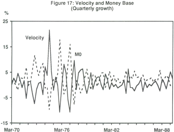
No stability tests have been conducted on M0. The monetary base appears to have no relationship to either nominal or real income over the short run. This can be seen by looking at the velocity of the monetary base (the ratio of nominal income to M0). If there is a connection between M0 and nominal income, velocity (V) should be stable and predictable. Figure 17 displays changes in M0 against the corresponding changes in velocity. As illustrated, an increase in M0 is almost exactly offset by a decrease in velocity. Equivalently stated, V behaves passively, so that a change in M0 has virtually no effect on income. The correlation between changes in M0 and changes in V is −0.907; this behaviour is the same after 1983 as before 1983, so that it is not attributable to one particular regime. It also exists in annual data (Milbourne (1990)) so that it is not attributable to the periodicity of the data. One of the points to arise in this context was the very poor performance of demand for M0 (or equivalently, velocity) equations. Taking a wide variety of dynamic specifications, Milbourne (1990) showed that the velocity residual was very highly correlated with the monetary base, which should not be the case if velocity can be well explained by standard variables.
Several authors, particularly Benjamin Friedman (1982), have argued that broad credit aggregates should be more closely related to economic activity. As HM show, this has not been the case for Australia. There are several reasons. First, broad aggregates do not capture all borrowing activity. Broad money includes recorded borrowing by the NBFIs. Other aggregates, such as credit, seek to capture lending to the private non-finance sector. However, there are other ways in which borrowing takes place which are not included in these figures. For example, inter-firm credit and household borrowing in the form of trade credit are not included, nor is borrowing between households (parents lending house deposits to their offspring, for example). Most measures do not include new equity issues, and no aggregate includes the retained earnings of firms (internal funds) which are generally the first committed to new investment projects. These funds are quite substantial. But perhaps of more concern is the use of off-balance-sheet business by the trading banks. This unrecorded intermediation has grown substantially in the last few years.
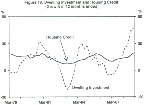
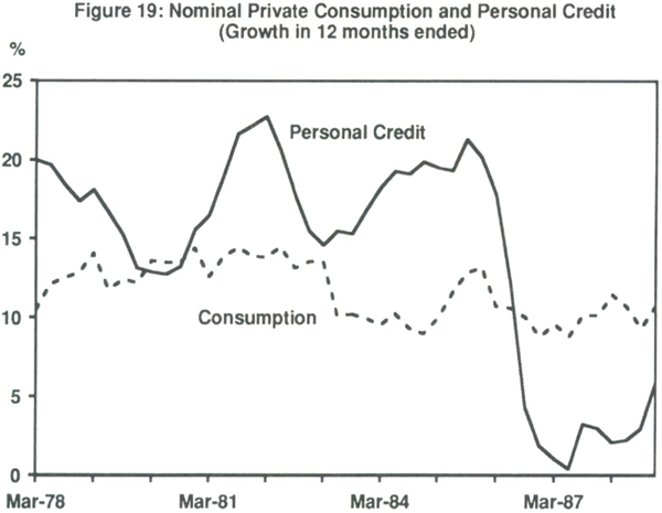
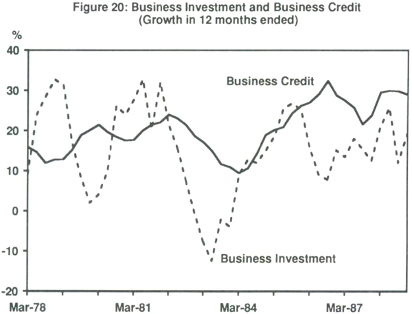
There is a deeper problem regarding the relationship between credit measures and economic activity. Probably reflecting the above points, credit on a disaggregated basis is unrelated to the relevant components of aggregate demand. This is illustrated in Macfarlane (1989a) and is reproduced below in Figures 18 to 20. A strong relationship between private consumption and personal credit, and between business credit and business fixed investment, is difficult to find. There appears to be some cyclical relationship between dwelling investment and housing credit. However, there does not appear to have been an upsurge in the provision of housing credit relative to the rise in dwelling investment in the last few years of the decade. It is therefore not surprising that there is little relationship between measures of recorded credit and economic activity.
5. Current Theoretical Issues in Monetary Policy
Three questions which arise in discussing the framework of monetary policy are:
- what is the ultimate objective of monetary policy?
- are these best achieved by the use of rules or discretion? and
- what is the role and/or optimal choice of an intermediate target?
How one answers these questions depends upon one's belief in the appropriate model for the Australian economy. Since this underlies most of the discussion of economic policy, it is useful to highlight this point by considering two extreme examples. Consider an extreme classical economy in which all prices are completely flexible, so that all markets clear, and there is perfect information. In this framework, neither fiscal nor monetary policy will affect output in the short run (they may affect output in the long run if they affect capital accumulation and labour via the tax system). Since a change in the money stock could not affect real output, it must only affect a nominal variable such as the price level (or its rate of change), which is therefore the only sensible ultimate objective. As shown by Lucas (1972), allowing for uncertainty and incomplete information does not alter this view, provided that expectations are correct on average (rational). In this case monetary policy cannot systematically affect real output and can only affect the price level. Thus a classical economist would select the price level as the ultimate objective of monetary policy, one of the definitions of the money stock as the intermediate target and whichever was the best tool to control that money stock measure (interest rates or the monetary base for example) as the instrument.
The key assumption of the extreme classical model is that prices are completely flexible. Now consider the other extreme – the Keynesian case where prices are rigid in the short run and respond to cost considerations rather than demand. In this scenario, a change in the money stock will change real output without affecting prices. Thus the only sensible ultimate objective of monetary policy can be real output. The intermediate target might be a financial variable, but it might also be the rate of unemployment if this is a better proxy for output. The instrument is likely to be the interest rate. In this case, monetary policy would respond to unwanted changes in real output – that is, it would be counter-cyclical. In the classical case the role of monetary policy is to control the price level, so that it would not respond to cyclical changes in output.
These two views of the world are not mutually exclusive; they may both be reasonable approximations over different time periods. Most macroeconomists have in mind an eclectic model which is Keynesian in the short run because there are various institutional features which make prices (including wages) slow to change, but classical in the long run as increases in output, following an increase in the money stock, exert demand pressures on the price level. What determines one's view about the appropriate instruments and objectives is then: “how long is the short run”.
However, as far as monetary policy is concerned, the real issue is: “how long is the short run relative to the lag in monetary policy?” If monetary policy takes 12 months before its effects are felt, yet disturbances rectify themselves within 6 months, then monetary policy might stimulate the economy at precisely the wrong time, thus de-stabilizing it. It is important to highlight this point because most theoretical analyses of monetary policy, which are often static, do not take into account the lags involved.
(a) Rules versus discretion in the conduct of monetary policy
One of the issues that has continued to be debated in the 1980s is whether the monetary authorities should stick to a fixed rule (say for monetary growth) which is independent of economic events, or whether monetary policy should be altered depending on the state of the business cycle. Monetary targeting is an example of a fixed rule in which the growth rate of the money supply is pre-announced and (supposedly) not altered. This policy prescription follows from a classical model in which the rate of inflation equals the rate of monetary growth, so that such a rule would control the inflation rate but have no effect on output.
An alternative policy is to have a known contingent rule, which specifies a given monetary policy for each set of circumstances. If the intention were to smooth the business cycle, a feedback rule would make the instrument – say the interest rate – dependent upon real income. More general rules might be established depending upon a number of variables or possible disturbances. (Some of these are discussed below). The difficulty is that capturing even the major disturbances adequately requires a contingent rule so complex that it would not be understood easily.
A third alternative is to have an unstated contingent rule, that is, to use discretion. One of the disadvantages of discretion is that there is no stated policy on which economic agents can base their actions or expectations. For example, if it is felt that the monetary authorities will not behave in an anti-inflationary manner, there is nothing to tie down expectations of inflation, which by itself may be sufficient to start an inflationary surge. The post-1985 “check-list” approach is an example of discretionary policy, and the debate over what RBA policy actually was (discussed in Section 3(e)) is an illustration of the problem.
(i) The argument for rules
There are four strong arguments advanced by those who advocate rules for monetary policy, which usually take the form of pre-announced rules for monetary growth. The first argument, discussed above, is that such a policy provides a firm anchor for expectations of inflation. The second argument is that a fixed rule gives a clear benchmark by which the performance of the monetary authorities can be judged. If, as occurred in Australia prior to 1985, the monetary aggregates grow at rates greater than announced, the monetary authorities can be seen to have failed. Thus the publication of growth targets creates the right incentives for the monetary authorities.
The third argument is that without rules, the government or monetary authority has an incentive to act in a dynamically inconsistent fashion, which leads to an inflationary bias in monetary policy (Barro and Gordon (1983)). Dynamic inconsistency occurs when the government reneges on a previously announced policy. An example might be a government which announces a tight (anti-inflationary) monetary policy, and induces people to believe in that policy. However, just before an election, the government has an incentive to pursue an expansionary policy, gaining a boost in real output, with the ensuing inflation hopefully coming after the election. This incentive to depart from a previously announced path causes a credibility problem for any government; a tight monetary policy might not be believed because all agents realize that it is in the government's interest not to keep to the bargain. Thus any government will have a credibility problem in convincing agents to believe that inflation will be kept down. Moreover, if agents realize the incentive scheme, they will come to expect inflation and will frame their wage demands accordingly, producing actual inflation. This imparts an inflationary bias to policy.[18]
A fourth reason for a fixed monetary growth rule is that it imposes discipline upon negotiators of wage bargains, for example. If the monetary authorities make clear that they will not underwrite inflation, wage bargains will limit the increase in nominal wages to avoid the large unemployment that high real wages would bring. This raises the point that even though monetary variables might not seem to influence prices, monetary policy might influence those variables that do influence prices. A known, believed commitment to low inflation might bring about lower rates of nominal wage increase than without such a commitment.
(ii) Arguments against fixed rules
The main argument against fixed monetary growth rules is that they fail to take account of shifts in velocity or structural changes. Thus changes in tastes, deregulations, and financial innovations, will produce misleading values for the monetary aggregates. Moreover, many of these changes cannot be forecast or even recognized for some time. There are three reasons for shifts in velocity, and it is important to distinguish between them.
One reason for shifts in velocity during the 1980s has been various innovations and deregulations. A second source of velocity shift has been such things as changes in tax legislation and tastes. The behaviour of velocity of most financial aggregates since 1985 (when most of the deregulations were completed) illustrates that this has been an important source of velocity shift. Both of these shifts can be considered as exogenous to the financial sector. They make monetary targeting difficult, but not impossible if the velocity shifts can be discovered quickly enough and accurately enough.
A third type of velocity shift does make monetary targeting impossible: shifts caused by the monetary targeting procedure itself. This is known as Goodhart's law, which is an example of the famous Lucas (1976) critique of economic policy. This says that empirical relationships between financial aggregates and other variables start to break down as soon as the authorities try to exploit them. In this case the shifts in velocity are endogenous. Consider the following example. Suppose that over a long period of time, water usage had been proportional to population, but insensitive to the price of water (which had been regulated), and suppose that this was an extremely good empirical relationship. Now suppose that, in a change of regime, a drought causes water to be rationed by half. According to our very good empirical relationship, half of the population will die. Clearly that is absurd; behaviour will change. The same story is likely to hold if “currency” replaces “water” and “income” replaces “population”. It is these endogenous changes in behaviour, or velocity, which are the most problematic. They will still be there even when deregulation has been finished.
A further issue is whether the monetary authorities should use an intermediate target, and if so, what. This issue is addressed in the next section.
(b) Intermediate targets: some general issues
The role of monetary policy hinges on the relationship between the instruments that the monetary authorities possess and those macroeconomic variables perceived to be the objects of monetary policy. Monetary authorities receive a flow of information at different time intervals and must interpret what these pieces of information imply about the future direction of the variables that they ultimately wish to influence or control. Much of these data – National Income data, for example – are received with a lag and the provisional data may contain a great deal of noise. As a result, the monetary authorities may choose to focus on and target an intermediate variable (or variables). Thus, a simple description of monetary policy might be:
monetary policy instrument → intermediate target → ultimate objective
There are three properties which an intermediate target should possess:[19]
- it should be observable with a short lag (observability);
- it should be controllable by the instrument variable (controllability); and
- it should have a predictable relationship with the ultimate objective, both in magnitude and timing (predictability).
Without these properties, an intermediate target may be inadvisable. For example, suppose that the instrument was the cash rate, the intermediate target was M3, and the ultimate target was the rate of inflation. If random shifts occurred in the demand for M3, both the relationships between the cash rate and M3, and between M3 and the rate of inflation, may be unstable and unpredictable, implying lack of monetary control. Yet there could exist a stable relationship between the cash rate and the rate of inflation which is usable for economic policy. In this case, it would be better to abandon the intermediate target altogether.
If an intermediate target is desirable, the question is: “which one?” This depends upon the type of shocks that are the most dominant and upon the ultimate objective. It is worthwhile to begin by considering the choice of targets using the analysis of Poole (1970). Poole considered a closed economy with fixed prices, and examined the question of what stabilization policies should be pursued in the case of two types of shocks: an exogenous shock to expenditure, and an exogenous shock to money demand (caused, for example, by a financial innovation).
Allowing both fiscal and monetary policy a role and assuming no policy lag, in the standard IS/LM analysis, shocks to expenditure will shift the IS curve. To avoid changes in either income or the interest rate, the best policy is to use fiscal policy in order to shift the IS curve back to its original position. In the case of a monetary disturbance, a shock which shifts the LM curve should be answered by an offsetting change in the money supply which shifts the LM curve back to its original position. Any other response – for example a monetary policy response to an expenditure shock – will result in volatility in either the interest rate or income.
If fiscal response is ruled out, as seems to be the case in Australia currently, the appropriate monetary response also depends upon which type of shock occurs. If we concentrate on the objective of stabilizing income, then an expenditure shock should be answered by an opposite (counter-cyclical) response in the money stock as shown in Figure 21a. A positive shock to the IS curve (IS0 to IS1) would result in income increasing from y0 to y1 unless the money stock was reduced (shifting LM0 to LM1). The penalty is an even higher interest rate than would have otherwise been the case. Notice that targeting (pegging) the interest rate in this circumstance would lead to an even-greater divergence of income than targeting the money stock would produce. In order to keep the interest rate at i0, the required increase in the money stock would shift LM to LM2, in which case income would rise to y2.
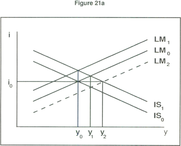
If the shock is monetary in nature (shifting LM0 to LM1 as in Figure 21b), then a policy of targeting the interest rate (thus reducing the money stock) would return LM to LM0, with no change in income. If the money stock is targeted (that is, left unchanged) then income would change from the desired y0 to y1. In summary, if only monetary policy is available, and the objective is to stabilize income, the money supply should be pegged if the shocks are to expenditure, and the interest rate should be pegged if the shocks are financial. This suggests that if most of the shocks during the 1980s were on the financial side, the interest rate should have been the intermediate target, not the money stock.
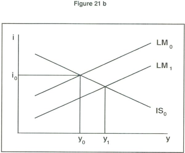
There are two important respects in which Poole's analysis is incomplete (in addition to ignoring lags): the neglect of both prices and open economy issues. It is easy to see that if we allow for flexible prices, pegging the interest rate is no longer an option. To see this, consider an increase in expenditure which raises the interest rate. Pegging the interest rate requires an increase in the money stock, so that income increases again. This increase in demand puts pressure on the price level, which raises the demand for money. To hold the interest rate constant, the monetary authorities must raise the money stock again, which continues the process. There is no price level at which the process will settle (that is, there is no determinate price level)[20] so that a fixed or pegged interest rate is not feasible. When open economy considerations are introduced, pegging the interest rate may not be an option either. In the case of uncovered interest parity, the domestic interest rate must equal the foreign interest rate plus the expected rate of depreciation of the currency. Since the monetary authorities cannot (perfectly) determine either of these, the scope of policy is limited.
Because M3 targeting became so difficult, and so unfashionable, some other variables have been nominated as possible intermediate targets. In the following subsections, the cases for and against each of these are briefly analysed, in terms of the three requirements of the intermediate target: observability, controllability, and the relationship to the ultimate objective of the intermediate target. One issue which will influence the last of these is the type of shocks that will be hitting the economy. In the literature on the issues of targeting, four potential shocks have been identified. These are aggregate demand shocks, financial sector shocks such as the demands for certain financial assets or financial innovations and deregulations, shocks to the terms of trade (which have been very important in the 1980s in Australia), and price shocks. The oil shocks of the 1970s were clearly examples of price or aggregate supply shocks, although these seem to have been less important in the 1980s.
(c) The choice of specific intermediate targets
(i) The monetary base
The monetary base clearly passes the test of quick observability, since it is available to the monetary authorities with the same timing as other monetary aggregates and interest rates. Targeting of the monetary base has been advocated for Australia by Sieper and Wells (1989), Porter (1989), McTaggart and Rogers (1989) and alluded to by Harper and Pearce (1989). On the issue of controllability, McTaggart and Rogers in particular claim that the monetary base would be much easier to control on a day-to-day basis than other monetary aggregates, provided there is a change in operating procedures (discussed above). This change of procedures would mean that the RBA would not act as a lender-of-last-resort; that is, they would deny liquidity to the banking system if a liquidity crisis arose.
The most problematic aspect is the relationship of the monetary base with income or the price level. As shown above in Figure 17, the velocity of the monetary base is very unstable, and tends to move inversely to changes in the monetary base itself. Even so, such a stable relationship would not be sufficient. A policy of targeting the monetary base would constitute a regime change which would change the nature of the relationship between the monetary base as intermediate target, and whatever is the ultimate objective. The primary issue of the past relationship of M0 to income is whether it has been caused by specific shocks, and whether these shocks are likely to occur and even if not, whether the relationship is stable enough to use.
One conclusion which can be generalised from Poole's analysis is that a monetary intermediate target is inappropriate if money demand is unstable. A qualification to this view has been given by Jonson and Trevor (1981) who argue on the basis of a dynamic version of Poole's analysis that even though the LM curve is unstable, it still may be better to fix the money stock because of less inflationary uncertainty. This argument relies on there being a relationship between monetary uncertainty and inflationary uncertainty, to which current evidence does not point. One of the reasons advanced for M0 is that it has not been affected by innovations and deregulations as much as other aggregates. Thus the lack of relationship with price and income is surprising.
There are two theoretical concerns with M0. One is that M0 does not include the reserves of NBFIs, so that a great deal of substitution could take place if the reserves (and thus activity) of the banks alone were controlled. A second concern is that M0 consists largely of currency, the demand for which might be changed by further financial innovations.
The following would be the response of the economy to the four types of shocks if M0 were targeted. For an aggregate demand or money demand shock, the analysis would be the same as Poole's. Monetary targeting would be better than interest rate targeting if shocks came mostly from aggregate demand, since it reduces income fluctuations and hence price level fluctuations via the Phillips curve. The reverse is the case if most of the shocks are financial in origin. For a terms of trade shock, an M0 target (if feasible) would not counteract the effects on income, but it would counteract changes in the price level (by not accommodating the inflationary effects which would follow from an exchange rate depreciation following a worsening in the terms of trade, for example). For a (positive) price or (negative) aggregate supply shock, a non-accommodating policy of keeping M0 fixed or on target would restrict the rise in the price level, but lead to a larger contraction in income. Thus, M0 targeting, if relationships are stable, leads in general to a lower variance in price, and a higher variance in output.
(ii) Credit
Credit has been advocated as one possible intermediate target mostly by proponents in the United States – for example Benjamin Friedman (1982). It is certainly observable quickly. However it has two main drawbacks. The first is its controllability, and the second is its relationship with income. Dealing with the second of these issues first, Figure 8 above and related discussion in Section 4(d) has shown that credit has had a particularly unusual and indeed unstable relationship with income, particularly over the last five years (see also Macfarlane (1989a)). In particular credit is a function of a number of factors which are not under control of the monetary authority – such as changes in tax regulations which induce firms to swap from equity to debt and vice versa. In addition, the findings of BMS and BST show that credit has at most a contemporaneous relationship with income, although there is more evidence that it lags nominal income. Thus it is not a particularly useful aggregate to target if the ultimate objective is either nominal income or one of its components, price or output.
Further work in the United States by Benjamin Friedman (1988) has concluded that credit is as unstable as any other monetary aggregate and he has abandoned his initial position. This duplicates findings of Home and Monadjemi (1985) who have documented those results for Australia. A final consideration is that actual measures of credit do not include the total available amount of credit; for example the data do not include equity, trade credit, or the off-balance-sheet items of the banks, which are now quite substantial. Credit targeting should have the same consequence for given shocks as M0 (unless the aggregates are affected differently by different financial shocks).
(iii) Nominal income
Many economists, beginning with Gordon (1985, written 1983) and Hall (1983), have advocated the use of nominal income as an intermediate target. The main disadvantage with nominal income targeting is its observability; data are not available as quickly for the financial aggregates. In addition, the initial estimate may be subject to some error. The second problem relates to its controllability. There are many factors and shocks that affect the value of nominal income but are outside the scope of the monetary authorities. This creates a problem of credibility if the RBA has set nominal income targets but then cannot deliver. The major advantage is the relationship between nominal income and the final target. There is a very close relationship in the short run between changes in nominal income and changes in real income. Thus if real income is the ultimate objective this aspect is a positive argument for the use of nominal income targets. There is also evidence that prices tend to lag changes in nominal income by approximately twelve months, and there is certainly a folklore that this relationship is stable, or certainly much more stable than most other empirical relationships between macro-economics variables.
What consequences would nominal income targeting have when the economy is subjected to shocks? The advantage is that this rule automatically protects against two particular types of shocks. The first is a financial shock. From the identity MV=PY, a shock to velocity will automatically imply an offsetting change in the money supply to keep nominal income on target. Clearly this is an advantage if most of the shocks in the system are thought to be in financial markets.
The second advantage, in a static framework, of a nominal income target is in the case of a price shock. The rule to target nominal income will automatically call for a reduction in the growth of real output to pull nominal output back into line. According to standard Phillips curve arguments, this would reduce pressure on the rate of inflation. Taylor (1985), however, claims that in a dynamic setting, the propagation effects are more important than the direct effects. Using a simple empirical model of the U.S. economy, Taylor finds that when lags are taken into account, the impact of price shocks on the business cycle is larger under nominal income targeting than under a monetary targeting regime. This is an example of how static analysis might be misleading.
A positive aggregate demand shock with nominal income targeting would produce a higher interest rate and/or an exchange rate appreciation. These variables would thus be more volatile on average than under a regime which smoothed the exchange rate or interest rate. This same conclusion would also be produced by a monetary target. A terms of trade shock, since it initially has opposite effects on price and output, would produce little response if nominal income were being targeted. This shock thus leads to volatility in price and output.
(iv) The exchange rate
One possible intermediate target is the exchange rate. Whilst many central banks might attempt to target the exchange rate in order to reduce volatility on a day-to-day basis, using the exchange rate as an intermediate target essentially implies pegging the exchange rate. Since the exchange rate is determined minute by minute, observability is instantaneous. Further, by appropriate buying and selling of foreign currencies each day, the RBA can peg the exchange rate at whatever level it wishes. Indeed, much of the literature on international monetary coordination and cooperation has focused on this issue, claiming that during the 1980s most of the central banks attempted through co-operative measures, to stabilise movements in the exchange rate (Goodhart (1989), OECD (1985)). The issue of monetary co-operation is surveyed in McKibbin (1988). The main advantage is that it ties expected inflation to that of a larger trading partner. The disadvantage is that if that larger trading partner does not experience the same types of shocks, it leads to major swings in output.
The main disadvantage in using the exchange rate as an intermediate target (but not neccessarily fixing it) is the relationship between the exchange rate and the ultimate policy objective. The authorities must know which exchange rate is the correct one, and whether the exchange rate is at its “fundamental” level. On the first point, the government cannot continue to peg the exchange rate at an inappropriate level forever. This is especially so because in an increasingly integrated international capital market, the possibility of currency substitution may lead to swings in demand for domestic currency and increased speculation. On the second point, the relationship between the exchange rate, the current account and income has been a major empirical puzzle to economists (Macfarlane and Tease (1989)). It is not clear that such a relationship can be relied upon.
The advantages of reduced volatility of the exchange rate is that it is good for investment and exports and, in the short run, price stability. The disadvantage is that control of monetary policy must be given up. Exchange rate targeting works well if the shocks are financial, and Blundell-Wignall and Gregory (1989) have argued for exchange rate targeting in this situation. For an aggregate demand shock, targeting the exchange rate leads to greater output variability because the money supply is endogenous and becomes accommodative. The effect on price variability is ambiguous because the reduced volatility of the exchange rate reduces price variability, but the reduced volatility of output increases price volatility.
Exchange rate targeting does not work well in the presence of terms of trade shocks. A flexible exchange rate partly offsets terms of trade effects upon income, just as relative price changes offset the effects of a reduction in demands for certain goods. Thus this regime would not be useful if policy was directed towards stabilizing income, and the predominant shocks were to the terms of trade. However, if the predominant shocks were to price, a policy that targeted the exchange rate would make monetary policy accommodative; this would minimize effects on income but would exacerbate effects on the price level.
(d) Contingent money supply rules
Edey (1989), and Stemp (1988, 1989a, 1989b) consider contingent rules for monetary policy when there is a variety of shocks. These papers extend the Poole analysis with both flexible prices and/or an open economy. The analysis of these papers confirms the original Poole finding – that if financial shocks (i.e. shocks to money demand and/or financial innovations and deregulations) are the dominant shocks, then a money supply rule is not optimal and either interest rates or the exchange rate or some other variable should be targeted. If financial shocks are not dominant, Stemp and Edey illustrate that it is possible to write down a rule setting the money supply as a function of observable variables. This appears to be a formal description of the checklist of variables where the money supply is adjusted depending on the values of the exchange rate, the income level, the price level and the interest rate. As expected, the weight given to any variable in this checklist depends upon its relative volatility. If a variable is “noisy” then it has less information content, and therefore will carry less weight in determining the optimal change in the money supply.
These contingent rules are quite complex since the coefficients of each of the variables in the rule depend upon the relative variances of each shock, on the parameters of the models, and on the ultimate objective. There are however a few intuitive results. The first is that if targeting income is the ultimate objective, then it is not possible to write down a general linear rule for the money supply that always keeps output on a pre-planned path when there are simultaneous shocks occuring. The second issue relates to whether the ultimate policy should allow for base drift. Base drift implies that past mistakes are not corrected; i.e. even if previous policy allowed a higher rate of inflation than expected, this does not alter current policy. The main conclusion is that if the object is to stabilise income, then the optimal policy is to allow for base drift – that is, not correct past mistakes. If however the objective is to stabilise the rate of inflation, then base drift should not be allowed. In this situation, monetary policy should react to an above-target inflation rate. The intuition of this argument is as follows. If current policy reacts to past inflation, then high inflation last period will imply a restrictive policy this period, which would reduce the current real money supply. This contracts output and reduces the rate of inflation (ignoring time lags). Clearly this helps in controlling inflation but not in controlling income.
Except for financial shocks – where the money supply is inappropriate to target – the appropriate money supply rule is not clear. This is because it depends upon parameter values. Consider a shock to the terms of trade which lowers income and induces an exchange rate depreciation. The falling income will act to reduce the rate of inflation but depreciation of the exchange rate will act to increase the rate of inflation. Which way the rate of inflation actually goes depends upon the relative strength of those effects. The ultimate objective of policy influences whether monetary policy should be expansionary under these circumstances. Without knowing the relative parameter values, and without knowing the relative variances of the shocks, it is impossible to frame an exact rule for how the monetary authority should react to such a terms of trade shock. Moreover, the dominance of various shocks changes over time, so that a rule with unchanging weights may not be appropriate.
(e) Monetary policy in a deregulated system
The financial deregulations of the 1980s have changed the operation of monetary policy from that discussed in Section 3(b) prior to deregulation. Deregulation has forced monetary policy to work via the price of assets rather than the quantity. This means that the interest rate plays a more important role in the conduct of monetary policy than before.
This does not mean that the RBA has less control over quantities. Clearly, the floating of the dollar and the new system for the sale of government bonds gives the RBA more control over the monetary base. This is useful only if monetary base control is a feature of monetary policy. If M3 is still regarded as the key monetary aggregate, the question is whether it can be usefully controlled via M0. Macfarlane (1989a) claims that the money multiplier (Figure 22) is too unstable for the RBA to use, a comment echoed for other countries by Dotsey (1987).
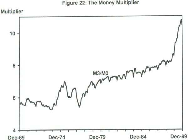
Since monetary policy operates via the cash rate, Morris (1988) suggests that deregulation makes control of monetary aggregates harder. In a deregulated world, with current deposits earning near-market rates of interest, all interest rates will tend to move together, which will lower the interest elasticity of money demand. If the returns to bank deposits differ from market rates only by the cost of exchange settlement, there may be a constant differential between interest rates on bank deposits and other (non money) assets. As a result, variations in the cash rate will not bring portfolio adjustments between money and other assets; their interest rates will rise and fall together.
How will deregulation affect the relationship between monetary variables and economic activity? Without direct restrictions on lending, Marsden, Healey and Doyle (1989) maintain that control of spending will be more difficult, and that without quantitative controls, control of lending will require a higher interest rate. This brings us to the question of whether the interest elasticity of investment is high enough for such control, and whether it has been affected by deregulation (and innovation). In particular, with fewer restrictions on banks' portfolio holdings, there will be less ability to affect the term structure of interest rates. Financial intermediaries will be free to convert instruments of any maturity into other maturities. Thus longer-term rates will be related to shorter-term rates by the expectations of future short rates. Monetary policy will then rely on expectations of more permanent changes in direction, rather than on direct intervention in interest rates of particular maturities.
Oster (1988) maintains that the interest elasticity of investment will fall as a result of the increased availability of floating rate loans relative to fixed rate loans. This argument is incorrect in a world in which the expectations theory of the term structure holds approximately, since fixed rates will reflect expectations of future rates. In particular, there is now an active swap market in which floating-rate liabilities can be exchanged for fixed-rate liabilities, and vice versa, in both domestic and foreign currencies. This makes the distinction between fixed and floating rate liabilities largely irrelevant. However, what is of interest is whether the elasticity of investment under the previously regulated, largely fixed-loan, system is higher than the elasticity that now prevails. This is not necessarily so. Under a fixed-rate system, old loans are not affected by higher current fixed rates, whereas new loans would be. Under a deregulated floating-rate system, both old and new loans would be affected, but probably by a numerically smaller amount than under the fixed-rate system, since the higher current interest rate may not be expected to last for the remaining maturity of all loans. Thus the answer depends upon the existing maturity structure and expectations, and there is no empirical evidence on this.
One issue which does arise in a deregulated system is whether monetary policy should address itself to the foreign (mostly private) debt, which has accumulated since the freeing of capital and credit controls. This problem is not a temporary one, and so the issue is whether monetary policy can solve a permanent problem, to which the standard answer is “no” for changes in levels of the money stock. Pitchford (1989) argues that the debt is no real economic problem, and thus it does not require a solution. Jonson (1989) and Kingston (1990) argue for a tightening of monetary policy as part (but not all) of the appropriate policy response. The primary aim is to reduce demand and so lower the current account deficit which adds to the debt. This cannot be a long-term solution unless it reduces tax distortions. Bowden (1989) argues that in the short run, a restrictive monetary policy makes the problem worse since it raises interest rates causing a capital inflow which increases the current account deficit; this in turn causes an expectation of currency depreciation which adds further upward pressure on the interest rate. The cycle is broken when aggregate demand eventually slows as a result of the restrictive policy.
An alternative is expansionary policy to lower the exchange rate in the hope of improving the trade balance. The problem with this policy is that interest payments will rise on debt which is denominated in foreign currencies if there is a depreciation, so that if it is not hedged overseas, both Australian domestic income and the current account will worsen. These considerations make it very unlikely that there is anything that monetary policy can do even if the debt is perceived as being a problem.
6. What Have We Learnt?
The conventional wisdom is that the 1970s taught us that attempts to fine tune the economy, or target a real variable, failed (Freedman (1989)), although this view was rejected by Modigliani (1977). There appear to be five lessons that the experience of the 1980s has taught us.
1. Variations in the money stock do not now appear to be the main impulse of business cycles.
The experience of the 1980s has not been kind to the view that business cycles are primarily a monetary phenomenon. This view was the main implication of the writings of Friedman and Lucas in the 1970s, who argued that either changes in the money stock were the primary cause of business cycles with long and variable lags (Friedman), or that unanticipated money was the main cause of cycles with short lags (Lucas). The 1980s have exhibited much less variance of real output growth, rates of inflation, and real rates of interest than the 1970s, even allowing for the major recession early in the decade. Corresponding to this lower volatility has been a greater volatility in monetary aggregates. This goes against the monetary propagation view.
The statistical evidence available seems to indicate that real shocks have been more important not only in Australia, but in most countries. This is the conclusion of the OECD (1985) survey of industrialized countries. Blundell-Wignall and Gregory (1989) find the same for Australia. Three pieces of evidence lend support to this view. First, the correlation between the terms of trade and output growth are too much of a coincidence to ignore. Secondly, the correlation and timing between the real interest rate and investment does not support a standard monetary transmission explanation. Thirdly, the negative correlation between income growth and inflation suggests the dominance of real supply shocks, which send output and prices in different directions.
2. Financial regulations were unneccessary for the conduct of monetary policy
The conventional view during the 1950s, 1960s, and 1970s was that regulations on the portfolios and behaviour of banks were neccessary for economic stability (Friedman (1960)). Yet the deregulations in Australia and elsewhere have not been associated with increased instability. The evidence that regulations helped monetary control is hard to find. The large number of regulations in existence prior to 1983 did not help the RBA meet its M3 targets from 1978 to 1983, as Figure 5 shows, although one could argue that the unwillingness of the RBA to create a credit crunch to offset M0 growth indicated a lack of attempt. But the lack of regulatory controls combined with the abandoning of monetary targets did not prevent a fall and stabilization in the rate of inflation. According to the standard view, the dramatic growth in credit creation which followed each deregulation should have led to an acceleration in the rate of inflation.
3. Innovations have been as important as deregulations in explaining the behaviour of financial aggregates
The strongest indications of this have been the behaviour of M3 and credit since 1985 when most of the deregulations had been effected. The growth rate of M3 dropped sharply in 1986 due to a switch to off-balance-sheet activities, for example. The surge in credit, and foreign borrowings by banks, have been helped by the creation of new financial instruments. These changes seem to have had as much of a quantitative effect as deregulation had in the first half of the decade. While banks continue to innovate to avoid regulations, technology and competition encourages innovations such as active swaps and options markets. Other “innovations” lying outside the financial sector (such as changes in tax treatment of debt instruments) have also had an impact upon financial aggregates.
4. Empirical relationships have not withstood the changes of the decade
The 1980s have reinforced the view that reliance on empirical relationships always entails error, particularly if it is assumed that those relationships are, or will remain, stable. It is difficult to uncover the effect of regime changes on these relationships because of the generally long lags and the lack of observation periods of each new regime. Without good empirical evidence, it is difficult to know how these relationships have changed. However, two examples illustrate that it is perceived that relationships have changed in the transmission mechanism. The first is the surprise that has been expressed at the failure (in terms of its timing) of high real interest rates to reduce expenditure in Australia in 1988/89, as evidenced by the Treasurer's own statements, and the continued current account deficit. Tight fiscal and monetary policies have not reduced expenditure as the textbooks suggest; it may be that we are headed for a late “hard” or even “crash” landing (with a number of casualties) rather than an early soft landing as might have been predicted. The second piece of evidence is the relationship between exchange rates and the current account (see Macfarlane and Tease (1989)) which is difficult to explain.
5. There is life after monetary targets
Monetary targets were seen as the only practical course of action from 1975 until the early 1980s. Even as late as 1983, “most central bankers saw no practical alternative to monetary targeting” (Eguchi and Suzuki (1985)). Those central bankers now seem to have changed their position as a result of the experience of the 1980s.
Argy et al (1989) discuss the experience of monetary targeting in several countries and conclude that the rate of inflation came down during the period of targeting, although there are a couple of notable exceptions (e.g. Canada and the U.S.). However, inflation has fallen in Australia, Canada, and the U.S. following the abandoning of monetary targets. This is a surprise to many economists who argued that there would be no anchor to expectations, and thus inflation would accelerate rather than fall, as has been the case.
The most striking example of this has been the U.S. In 1983, Milton Friedman (1985, written 1983) took a very strong and public position about the future course of inflation. He predicted a major blowout in the rate of inflation to begin in 1984 because the Fed had allowed double-digit rates of monetary growth after abandoning targets in 1981. To Friedman's surprise, the rate of inflation fell below 4 per cent and stayed there, and there is no sign, some seven years later, of Friedman's prediction being correct. If lags are long and variable, they have become very long and very variable. The disconnection of growth rates of monetary aggregates, economic activity, and inflation has been one of the puzzles thrown up by the 1980s. But the important aspect of this example is that it illustrates that monetary targeting is not neccessary for credibility (although it still may be desirable) or for reducing inflation. The experience in Australia would lend support to this.
7. Where Do We Go From Here?
Monetary policy is currently in a state of uncertainty. The major problem is that monetary aggregates have proved unreliable either as targets or indicators. M3 and the broader aggregates lag income rather than lead income. The only aggregate which does lead income is M1, but this has been endogenous in any case, and it is likely that such a relationship will evaporate if it is exploited. Other possible targets have major problems. Nominal income data are received with a long lag and with some imprecision. Targeting the exchange rate increases vulnerability to aggregate supply shocks, such as productivity or terms of trade shocks. Additionally, the lags in monetary policy are long enough to raise debate about the circumstances under which monetary policy should respond to economic developments.
Given the apparent lack of success in targeting either real or nominal variables over the last two decades, the instability of monetary aggregates, and the relative importance of real shocks in the propagation of business cycles, what is the appropriate framework for monetary policy in the 1990s? The major questions would appear to be: (i) whether the RBA should set rules or targets or neither; (ii) how monetary policy should be presented to the public; (iii) what variables should be the main focus of RBA policy; and (iv) should the RBA respond to shocks, and if so, how. These questions are all interrelated.
The main arguments for fixed rules are theoretically appealing, but they suffer from major practical difficulties. It makes no sense to continue with a fixed rule for the monetary stock in the face of known permanent shifts in velocity, for example. Because people know this, and because they know that history has been littered with major fluctuations in velocity, any announcement of a fixed monetary rule would simply not be credible, which would destroy the main advantage to a fixed rule. The same would occur if the fixed rule was on the exchange rate. Exogenous disturbances which are semi-permanent make support for a fixed exchange rate impossible. Since this is known, and history has told us that terms of trade shocks are important, people will know that a fixed exchange rate is not credible, so a pre-announcement does nothing for credibility. Even a specified contingent rule on the exchange rate does not help since it may increase speculation which will cause wild swings in the monetary base. Tobin (1985) has made the point that governments, being what they are, cannot ignore a major recession (nor should they in his view) so that any sensible policy must take this into account. Of course one could argue that a constitutional amendment could prevent governments from changing rules. But any constitutional amendment can itself be amended if the situation dictates (such as unexpected changes in the structure of the economy). Because of these considerations, and because governments would ignore advice to the contrary anyway, I regard a fixed rule as totally impractical.
Given this, the issue is how the RBA should present its policy to the public. Clearly, the main focus of policy should be an anti-inflationary one over a longer-term horizon. Because the evidence is so strong that inflation in Australia is affected by a number of factors in the short run over which the RBA has little control, official inflation “projections” over the short term will involve credibility problems. It is important that the RBA makes a statement that it will not accommodate inflation in the 1990s at the same rate as in the 1980s so as to condition wage increases, for example. Provided an anti-inflationary policy is believed, it does not have to take the form of a fixed rule (as the U.S. and other examples this decade illustrate).
The above does not imply that the RBA should respond to every development. There is ample evidence from the Annual Reports that the RBA has become obsessed about world and Australian economic events, to the point of mentioning how and why the RBA responded to each event on a month-by-month basis. This is absurd, because it contains the implicit assumption that monetary policy works quickly enough to alleviate month-to-month problems. Whilst econometric estimates may not be very precise, it is statistically implausible that monetary policy lags are that short.
This leaves open the questions of what shocks monetary policy should respond to, and what variables the RBA should take notice of (in either an instrument or indicator capacity). Clearly, if shocks to the economy are permanent, there is nothing that monetary policy can do, except perhaps ease the transition to the new “equilibrium”. However, in practice, knowing what transition policy is the correct one (given the associated lags) is difficult, and it should be up to proponents of temporary intervention in the face of a perceived permanent shock to establish their case.
Thus the case for responding to shocks relies on a good knowledge of their effects and timing. It is silly to argue for a monetary rule unresponsive to shocks. Consider a rule which did not allow variations in the monetary base (or any monetary aggregate) over the Christmas period, with a resulting “credit crunch” every Christmas. Those who would advocate such a rule would be ignoring the biggest factor in the founding of the Federal Reserve and the reduction in financial panics (Miron (1986)). Of course, Christmas is a known “shock” with known time interval. For most shocks, the time interval is uncertain. It is this which makes monetary policy difficult.
As is clear from the discussions in Section 5, appropriate monetary policy depends upon what are the likely sources of shocks, and there is no simple policy prescription even if it is known whether low output variance or low price-inflation variance is preferred. It would be helpful to know in advance which shock is likely to be dominant. This is impossible to forecast, since the major changes or shocks have been different every decade. Three potential sources of shocks are:
- a wages breakout;
- further terms of trade shocks; and
- further innovations in intermediation and the payments mechanism.
The first two are aggregate supply shocks. The Accord has been in operation for seven years, during which time there has probably been less relative wage change than shifts in product demand would dictate. It is possible that restructuring of awards, or pressure from workers who feel that they have borne the brunt of wage moderation, will lead to a wage breakout. Further terms of trade shocks are likely to follow from recent events in Eastern Europe, which may lead to relative price changes between agricultural and manufacturing goods.
Recent monetary policy in the industrialized countries has been directed towards stability in exchange rates. In both supply shocks above, a fixed exchange rate policy would lead to dramatic changes in output and the current account, but not in the rate of inflation in the short run (since there would be no additional depreciation or appreciation effects). Letting the exchange rate adjust affects the rate of inflation in the short run, although not in the long run (when the price level has stabilized). If there were no bias to policy (e.g. pegging the wrong exchange rate), neither choice has any difference for the long-run rate of inflation. If these are the major sources of shocks, the choice becomes simple: go with flexible exchange rates and broad long-run monetary growth targets if output variance is to be avoided; go with exchange rate targeting if the concern is with short-run variability in inflation rates and if there is good knowledge of the appropriate long-run exchange rate.
There are at least four potential financial innovations. The first two are continuations of shocks occurring this decade: debt/equity changes resulting from fiscal and other policies, and switches between direct financing and intermediated financing. Both of these have an impact upon broader aggregates. Two further innovations are in the means of exchange. Currency demand will be affected by changes in automatic payments systems. In the extreme case in which all payments could be directly debited against a central account, the demand for currency would be zero (Harper (1984)). A second possibility is the removal of the RBA's monopoly on the issue of currency; that is, a return to the monetary system of Australia in the 19th century. Private issue of currency, as well as innovations in payments, would make the monetary base useless in its relation with income. Such developments might occur, with or without RBA approval. These are very powerful arguments against leaning on monetary aggregates as the main basis of monetary policy. Under these scenarios, monetary aggregates would be neither useful targets nor useful indicators.
If these predictions are correct, namely that the main shocks will be either supply based or financial, then an appropriate policy would be to respond to medium term shocks only (so that monetary policy has time to be effective). If, as I suspect, monetary aggregates will be hard to interpret and if sufficient lead time is available on supply shocks, then one policy would be to adjust interest rates directly in response to future expected changes in income or prices depending on which the government views is the flavour of the month. A policy which adjusts interest rates to inflation, for example, may be sufficient to anchor inflationary expectations. This after all, should be the key objective of monetary policy in the 1990s.
Footnotes
University of New South Wales. The author would like to thank Matthew Cumberworth for invaluable research assistance. Extensive comments from Geoff Kingston and Glenn Stevens are gratefully acknowledged. [*]
The original Phillips curve was a relationship between unemployment and the rate of change of wages. This relationship has been transformed into one between output and the rate of inflation. [1]
See Grenville (1989), for example. [2]
This process had been done for treasury notes in 1979. [3]
This is the case provided that the RBA controls its lending to the banks, an issue discussed in Sections 3(e) and 5(c(i)). [4]
RBA Bulletin November 1989, p. 14. [5]
In 1981, domestic deposits as a percentage of total liabilities were 71 per cent. In 1988, that number was 38 per cent (Linklater (1989)). Linklater, Mohl (1988) and Hogan (1989) discuss the changes in the structure of financial institutions post-deregulation. [6]
A summary of the debate about monetary targeting in the U.S. is contained in McCallum (1985). [7]
Argy et al (1989) do not view the policy makers of other countries as being very doctrinaire. [8]
Since OMOs involve a swap of money for bonds we ignore wealth effects for exposition. This can be justified using the arguments of Wallace (1981). Oster (1988) emphasises wealth effects in his discussion of OMO. However, the standard estimates of the effects of wealth on consumption are much less than the effects of income on consumption. [9]
A good survey of recent theories of how monetary policy affects output is given in Blanchard (1987). [10]
Unless workers have an employment protection feature in their agreement. [11]
Efficient capital markets imply that the interest differential between domestic and foreign assets should be equal to the expected rate of exchange depreciation, an unbiased predictor of which can be found from the forward rate. Empirical tests of this hypothesis (Smith and Gruen (1989)) do not fare well. [12]
Failure to do so would bring either a capital loss, or the opportunity cost of no capital gain. [13]
Unless all interest rates move together. [14]
Investment might also be related to short-term interest rates (if short-term loans are rolled over). However, the correlations with short-term rates are similar. [15]
The ambiguity of findings with respect to M1 is also discussed in Macfarlane (1989b). [16]
Veale, Boulton and Tease (1985) and Swamy and Tavias (1989) also investigate demand for money functions. These studies are not concerned statistically with the issue of stability. [17]
A survey of this literature is contained in MacDonald and Milbourne (1990). [18]
These are discussed by Parker (1989). [19]
A simple exposition of this indeterminacy is given in Edey (1989). [20]
References
Ando, A., Hidekazu, H., Farmer, R., and Suzuki, Y. (1985) (eds.), Monetary Policy in Our Times, Proceedings of the First International Conference held by the Institute for Monetary and Economic Studies of the Bank of Japan, MIT Press, Cambridge, Massachusetts.
Argy, V., Brennan, T. and Stevens, G. (1989), “Monetary Targeting: The International Experience”, Economic Record, 66, pp. 37–72.
Australian Financial System Inquiry (1981), Final Report, AGPS, Canberra.
Australian Financial System Inquiry (1982), Commissioned Studies and Selected Papers, AGPS, Canberra.
Australian Financial System Inquiry (1983), Report of the Review Group, AGPS, Canberra.
Barro, R.J. and Gordon, D. (1983) “Rules, Discretion, and Reputation in a Model of Monetary Policy”, Journal of Monetary Economics, pp. 12, 101–121.
Battellino, R. and Macfarlane, I.J. (1987), “Open Market Operations – Some International Comparisons”, Bulletin, December, pp. 1–10.
Battellino, R. and McMillan, N. (1989), “Changes in the Behaviour of Banks and their Implications for Financial Aggregates”, Reserve Bank Research Discussion Paper 8904.
Black, F. (1970), “Banking and Interest Rates in a World Without Money”, Journal of Bank Research, Autumn, pp. 9–20.
Blanchard, O.J. (1987), “Why does Money Affect Output?: A Survey”, National Bureau of Economic Research (NBER), Working Paper No. 2285, Cambridge, NBER.
Blundell-Wignall, A. and Thorp, S. (1987), “Money Demand, Own Interest Rates and Deregulation”, Reserve Bank of Australia Research Discussion Paper 8703.
Blundell-Wignall, A. and Gregory, R. (1989), “Exchange Rate Policy in Advanced Commodity Exporting Countries: The Case of Australia and New Zealand,” Paper prepared for the International Conference on “Exchange Rate Policy in Selected Industrial Countries”, 12–14th October, 1989.
Boulton, L.F. and Tease, W.J. (1984), “Financial Innovation Bibliography”, Reserve Bank of Australia, Research Discussion Paper 8402.
Bowden, R.J. (1989), “The Current Account and Signal Instability: Why the Monetary Cure Almost Kills the Patient”, University of New South Wales Working Paper, October.
Bullock, M., Morris, D. and Stevens, G. (1988), “The Relationship between Financial Indicators and Activity: 1968–1987”, Reserve Bank of Australia, Research Discussion Paper, 8805.
Bullock, M., Stevens, G. and Thorp, S. (1988), “Do Financial Aggregates Lead Activity: A Preliminary Analysis”, Reserve Bank of Australia, Research Discussion Paper, 8803.
Carmichael, J. (1990), “Inflation in Australia: Performance and Policy”, this volume.
Chapman, B.J. (1990), “The Australian Labour Market”, this volume.
Davis, K. (1988), Australian Monetary Policy: A Decade of Change”, Economic Papers, 7(1), pp. 1–15.
Davis, K. and Lewis, M.K. (1978), “Monetary Policy” in Gruen, F.M. (ed.), Surveys of Australian Economics, 1.
Davis, K. and Lewis, M.K. (1980), Monetary Policy in Australia, Longman Cheshire, Melbourne.
Dotsey, M. (1987), “The Australian Money Market and the Operations of the Reserve Bank of Australia: A Comparative Analysis”, Federal Reserve Bank of Richmond Economic Review, September/October.
Edey, M. (1989), “Monetary Policy Instruments: A Theoretical Analysis”, Reserve Bank of Australia, Research Discussion Paper 8908.
Edey, M. and Britten-Jones, M. (1990), “Saving and Investment”, this volume.
Eguchi, H. and Suzuki, Y. (1985), “Introduction” in Ando et al. (1985).
Fama, E. (1980), “Banking in the Theory of Finance”, Journal of Monetary Economics, 6, pp. 39–57.
Fama, E. (1983), “Financial Intermediation and Price Level Control”, Journal of Monetary Economics, 12, pp. 7–28.
Freedman, C. (1989), “Monetary Policy in the 1990's: Lessons and Challenges”, Paper presented to the Economic Policy Symposium, Federal Reserve Bank of Kansas City, 30 August-1 September 1989.
Friedman, B.N. (1982), “Money, Credit and Non-financial Economic Activity: An Empirical Study of Five Countries”, NBER Working Paper No. 1033.
Friedman, B.N. (1988), “Targets and Instruments of Monetary Policy”, NBER Working Paper No. 2668.
Friedman, M. (1960), A Program for Monetary Stability, Fordham University Press, New York.
Friedman, M. (1968), “The Role of Monetary Policy”, American Economic Review, pp. 1–17.
Friedman, M. (1985), “Monetarism in Rhetoric and in Practice” in Ando et al.
Garman, D.M. and Richards, D.J. (1989), “Policy Rules, Inflationary Bias and Cyclical Stability”, Journal of Money, Credit & Banking, 21 A, pp. 409–421.
Goodhart, C.A.E. (1989), “The Conduct of Monetary Policy”, Economic Journal, 99, June, pp. 293–346.
Gordon, R.J. (1985), “The Conduct of Domestic Monetary Policy” in Ando et al., pp. 45–81.
Grenville, S. (1989), “The Operation of Monetary Policy”, Paper presented to the Melbourne Money and Finance Conference, November 25–26.
Hall, R.E. (1983), Macroeconomic Policy under Structural Change, Industrial Change and Public Policy, Federal Reserve Bank of Kansas City.
Harper, I. (1984), “Some Speculation on the Long-term Implications of Financial Deregulation and Innovation”, Economic Papers, pp. 1–8.
Harper, I. (1988), “The SRD Requirement and Monetary Policy”, The Economic Record, September, pp. 178–186.
Harper, I. and Pearce, J. (1989), “Implementing Monetary Policy in an Era of Budget Surpluses”, Paper presented to the Melbourne Money and Finance Conference, November 24–25.
Hogan, W. (1989), “The Entry of New Banks in Australia”, paper presented to the Second Australasian Banking and Finance Conference, University of New South Wales.
Horne, J. and Monadjemi, M. (1985), “Debt, Credit, and Monetary Targeting in Australia”, Economic Record, 61, June, pp. 522–34.
Johnston, R.A. (1985), “Monetary Policy – The Changing Environment”, Reserve Bank of Australia Bulletin, June.
Jonson, P.D. (1989), “Australia's Balance of Payments: What is to be Done?”, Economic Papers, 8(4), pp. 33–40.
Jonson, P.D. and Trevor, R. (1981), “Monetary Rules: A Preliminary Analysis”, Economic Record, June, pp. 150–167.
Kingston, G. (1990), “Stabilising External Debt: Twin Deficits versus Tight Money”, Forthcoming in Kearney, C. and McDonald, R. (eds.), Recent Developments in Australian Monetary Economics.
Linklater, J. (1989), “The Structural Response of Financial Intermediaries to Deregulation – A Balance Sheet Approach”, Reserve Bank of Australia, Occasional Paper No. 11.
Lucas, R.E. (1972), “Expectations and the Neutrality of Money,” Journal of Economic Theory, 4, April, pp. 103–124.
Lucas, R.E. (1976), “Econometric Policy Evaluation: A Critique”, in Brunner, K. and Meltzer, A. (eds.) The Phillips Curve & Labour Markets, Carnegie-Rochester Conference Series, 1, pp. 19–46.
MacDonald, R. and Milbourne, R. (1990), “Recent Developments in Monetary Theory,” in Greenaway, O., Bleaney, M. and Stewart, I. (eds.) Economics in Perspective, Routledge Publishers, London.
Macfarlane, I.J. (1989a), “Money Credit and the Demand for Debt”, Reserve Bank Bulletin May, pp. 21–31.
Macfarlane, I.J. (1989b), “Policy Targets and Operating Procedures: The Australian Case”, Paper presented to the Federal Reserve Bank of Kansas City's Symposium “Monetary Policy Issues in the 1990s”, 30 August/1 September.
Macfarlane, I.J. and Tease, W. (1989), “Capital Flows and Exchange Rate Determination”, Reserve Bank of Australia, Discussion Paper 8908.
McCallum, B.T. (1985), “On Consequences & Criticisms of Monetary Targeting”, Discussion Paper, Carnegie-Mellon University.
McKibbin, W.J. (1988), “The Economics of International Policy Co-ordination,” Economic Record, 64(187), pp. 241–253.
McTaggart, D. and Rogers, C. (1989), “Monetary Base Control in Australia”, Paper presented to the Melbourne Money and Finance Conference, November 25–26, 1989.
Marsden, J.S., Healey, G.A. and Doyle, C.F. (1989), “Monetary Policy: A Structural Analysis”, Paper presented to the Melbourne Money and Finance Conference, November 24–25, 1989.
Marsden, J.S. and Jones, P.L. (1988), “Monetary & Exchange Rate Policy: A Volatility Based Perspective”, Economic Papers, 7(1), pp. 82–93.
Milbourne, R. (1985), “Distinguishing Between Australian Demand for Money Models, Australian Economic Papers, 24, 44, June.
Milbourne, R. (1986), “Financial Innovation, Deregulation and The Redefinition of Monetary Aggregates”, University of New South Wales Working Paper, No.91.
Milbourne, R. (1990), “The Money Stock, Velocity & Random Walks”, University of New South Wales, Mimeo, January.
Miron, J.A. (1986), “Financial Panics, the Seasonality of the Nominal Interest Rate, and the Founding of the Fed,” American Economic Review, 76(1), pp. 125–140.
Modigliani, F. (1977), “The Monetarist Controversy or, Should We Forsake Stabilization Policies?”, American Economic Review, 67, March, pp. 1–1a.
Mohl, A. (1988), “Patterns of Financing Post-Deregulation,” Economic Papers, 7(1), pp. 51–64.
Morris, D. (1988), “Monetary Transmission in a Deregulated Financial System”, Reserve Bank Research Discussion Paper 8811.
Moses, C.J. (1983), “Financial Innovations and Monetary Policy: A Preliminary Survey”, Reserve Bank of Australia Research Discussion Paper 8301.
O.E.C.D. (1985), “Exchange Rate Management and the Conduct of Monetary Policy,” Monetary Studies Series.
Oster, A. (1988), “Lags & Monetary Policy”, Economic Papers, 7(1), pp. 41–50.
Pagan, A.R. and Volker, P.A. (1981), “The Short-run Demand for Transactions Balances in Australia”, Economica, 48.
Parker, D. (1989), “Monetary Policy Under Deregulation”, Paper presented to the Melbourne Money and Finance Conference, 24–25 November.
Pitchford, J.D. (1989), “Does Australia Really Have a Current Account Problem?”, Economic Papers, 8(4), pp. 25–32.
Poole, W. (1970), “Optimal Choice of Monetary Policy Instruments in a Simple Stochastic Macro Model”, Quarterly Journal of Economics, 84, pp. 197–216.
Porter, M. (1979), “Money and Finance: The Direction of the Capital Market in the 1970's”, in Norton, W.E. (ed.), Conference in Applied Economic Research, Reserve Bank of Australia,.pp. 62–99.
Porter, M. (1982), “Monetary Targeting”, Australian Financial System Inquiry, Commissioned Studies and Selected Papers, Part I, 29–119, Australian Government Publishing Service.
Porter, M. (1989), “Monetary Policy” in Freebairn, J., Porter, M. and Walsh, C. (eds.) Savings & Productivity, Allen & Unwin.
Reserve Bank of Australia (1979–89), Annual Reports.
Reserve Bank of Australia Bulletins, 1979–1989.
Reserve Bank of Australia (1987), “Banking-Post Deregulation: The Australian Experience”, Bulletin, 1979–1989.
Richards, T. and Stevens, G. (1987), “Estimating the Inflation Effects of Depreciation”, Reserve Bank of Australia Research Discussion Paper 8713.
Sargent, T.J. and Wallace, N. (1982), “The Real Bills Doctrine versus the Quantity Theory: A Reconsideration”, Journal of Political Economy, 90, pp. 1212–36.
Sheilds, B. (1988), “Australian Monetary Policy: A Decade of Change”, Economic Papers, 7(1), pp. 16–33.
Sieper, E. and Wells, G. (1989), “Macroeconomics on the Left”, Paper presented to the Economic Policy Conference, Australian National University, November 27–28.
Smith J. and Gruen, D.W.R. (1989), “A Random Walk around the $A: Expectations, Risk, Interest Rates and Consequences for External Imbalance”, Reserve Bank of Australia Discussion Paper 8906.
Stemp, P.J. (1988), “Optimal Weights in a Checklist of Monetary Indicators”, Centre for Economic Policy Research Discussion Paper No. 192, ANU.
Stemp, P.J. (1989a), “Optimal Money Supply Rules Under Asymetric Objective Criteria”, Australian National University Working Paper, No. 186.
Stemp, P.J. (1989b), “Optimal Base Drift: Robustness Under Alternative Scenarios”, Australian National University, Mimeo.
Stemp, P.J. and Murphy, C.W. (1990), “Monetary Policy in Australia: The Conflict between Short-term and Medium-term Objectives”, mimeo, A.N.U.
Stevens, G., Thorp, S. and Anderson, J. (1987), “The Australian Demand Function for Money: Another Look at Stability”, Reserve Bank of Australia Research Discussion Paper 8701.
Stevens, G. and Thorp, S. (1989), “The Relationship Between Financial Indicators and Economic Activity: Some Further Evidence”, Reserve Bank Research Discussion Paper 8903.
Swamy, P.A.V.B. and Tavlas, G.S. (1989), “Financial Deregulation, the Demand for Money, and Monetary Policy in Australia, International Monetary Fund Staff Papers, March, 36, pp. 63–101.
Taylor, J.B. (1985), “What Would Nominal GNP Targeting Do to the Business Cycle?” in Brunner, K. and Meltzer, A. (eds.), Understanding Monetary Regimes, 22, North Holland, Amsterdam, Elsevier Science Publishers, BV, North Holland.
Tease, W. (1990), “The Balance of Payments”, this volume.
Tobin, J. (1985), “Monetary Policy in an Uncertain World” in Ando et al.
Valentine, T.J. (1982), “Monetary Targeting Revisited”, Bulletin of Money, Banking and Finance, 1982–83, (2).
Veale, J.M., Boulton, L.F. and Tease, W.J. (1985), “The Demand for Money in Australia: A Selective Survey and Some Updated Results”, in Meeting on Monetary Issues, Reserve Bank of Australia Research Discussion Paper 8502, November.
Wallace, N. (1981), “A Modigliani-Miller Theorem for Open-Market Operations,”, American Economic Review, June, pp. 267–274.