Bulletin – March 2014 Australian Economy Exchange Rate Movements and Economic Activity
- Download the article 1.6MB
Abstract
This article discusses estimates of the effect of movements in the real exchange rate on economic activity and inflation in Australia. The range of estimates suggests that a temporary 10 per cent depreciation of the exchange rate increases the level of GDP temporarily by ¼–½ per cent over one to two years. A permanent 10 per cent real depreciation is estimated to increase the level of GDP by around 1 per cent after two to three years and to increase year-ended inflation by ¼–½ percentage point over the same period. At an industry level, unsurprisingly, activity in trade-exposed industries is found to be more affected than in domestically oriented industries.
Introduction
Since the float of the Australian dollar in 1983, there have been large swings in the nominal exchange rate. In large part, these changes in the exchange rate reflect its role in cushioning the Australian economy from shocks. Since 1983, the exchange rate has appreciated or depreciated by 10 per cent or more over the preceding 12 months around one-quarter of the time. The real exchange rate (which accounts for differences in inflation rates across countries) experiences swings of a similar magnitude as most of the movements in the real exchange rate over horizons of one or two years can be explained by changes in the nominal exchange rate. Changes in the exchange rate of this magnitude – especially if they are sustained – can have significant effects on the real economy.
The exchange rate affects the real economy most directly through changes in the demand for exports and imports. A real depreciation of the domestic currency makes exports more competitive abroad and imports less competitive domestically, thereby increasing demand for domestically produced goods. Offsetting this to some extent is the effect of the higher cost of imported goods that cannot be substituted for domestically produced goods, including intermediate and capital goods required for the purposes of production. However, in most economies, the first effect is likely to dominate the second effect.[1] These effects do not occur immediately, but usually take several years to pass through the economy.
While the direction of the effect of movements in the exchange rate on the economy seems clear – with a depreciation usually associated with an expansion in activity and a rise in prices – the size of the effect and the sectors of the economy through which it is transmitted are less certain. This article reviews estimates of the effect of exchange rate movements on output and inflation, based on a range of models. One of these models also allows analysis of how exchange rate movements affect output in different parts of the economy, assessing which industries are more sensitive to the exchange rate than the economy as a whole.
In order to concentrate on the effect of the exchange rate only, in this article the exchange rate is assumed to change exogenously, that is independently from changes in other macroeconomic variables. However, the exchange rate frequently moves in reaction to other developments in the economy, such as changes in the terms of trade, the domestic or global outlook for growth, or interest rate differentials. In all these cases, the combined effect will be different from the estimates presented here. For instance, if the exchange rate depreciation occurs alongside a fall in the terms of trade, the expansionary effect of the depreciation may only partially offset the contractionary impetus of the fall in the terms of trade. Such scenarios can in principle be analysed with a number of the models presented here, but are beyond the scope of this article.
The Exchange Rate and Aggregate Output
In order to identify the effect of movements in the real (trade-weighted) exchange rate on output, a model that controls for contemporaneous changes in other variables which can also affect activity is required. The estimated effect of exchange rate movements on GDP is likely to depend on the model chosen, and on whether the change in the exchange rate is assumed to be temporary or permanent. In this article the results from a range of models are compared. The models chosen are a structural vector auto regression (SVAR) model based on Lawson and Rees (2008); a dynamic stochastic general equilibrium (DSGE) model based on Jääskelä and Nimark (2011); and estimates derived from separate models of exports and imports. All these models include lags of variables to account for the protracted nature of the pass-through of exchange rate changes. More details about the models are provided in Appendix A.
Table 1 summarises the estimates from these models. The first set of results suggest that a temporary depreciation – in which the real trade-weighted exchange rate index (TWI) depreciates by 10 per cent and then gradually returns to its initial level over approximately two years – increases the level of GDP by around ¼–½ per cent over one to two years, before it gradually returns to its initial level. The second set of results show that the effect of a permanent depreciation is larger, raising the level of GDP permanently by around 1 per cent after two to three years. This implies that GDP growth over these two years is (cumulatively) higher by around 1 percentage point than it would have been otherwise.
| Model | Temporary change in the exchange rate | ||
|---|---|---|---|
| Peak effect on level of GDP Per cent |
Peak Timing Quarters after depreciation |
||
| SVAR | 0.3–0.6(a) | 4–6 | |
| DSGE | 0.4 | 2 | |
| Permanent change in the exchange rate | |||
|
Effect on the level of GDP Per cent |
Number of quarters for three-quarters of total effect to occur |
||
| Model | After two years | Total effect | |
| SVAR | 0.7–0.9 | 0.9–1.1 | 7–9 |
| DSGE | 0.9 | 0.9 | 3 |
| Export and Import | 1.2 | 1.4 | 2 |
|
(a) The results from the SVAR model depend on how many lagged changes are included; see Appendix A Source: RBA |
|||
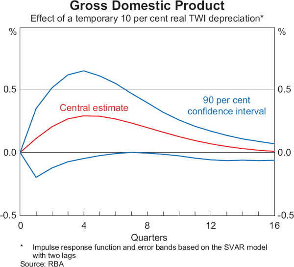
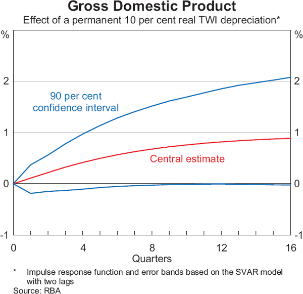
These estimates vary across the different models, but they are also subject to estimation uncertainty within each model. Confidence intervals are one way to illustrate how well an estimate fits the data, and therefore how likely it is that the true value is near that estimate. Graphs 1 and 2 illustrate this uncertainty with confidence intervals around the effect on the level of GDP of a 10 per cent depreciation for the SVAR model. In the case of a temporary depreciation, the 90 per cent confidence interval for this effect is 0–¾ per cent after about one year. In other words, even though the effect is most likely 0.3 per cent (the ‘point estimate’), there is a 90 per cent probability that the ‘true’ effect is between 0 per cent and ¾ per cent after about one year. In the case of a permanent shock, the confidence interval for the effect is 0–1½ per cent after two years.
The Exchange Rate and Industry Activity
Different industries are more or less sensitive to exchange rate movements and so the impact on the output of individual industries is likely to be larger or smaller than the aggregate effects reported above. Since much of the first-round effect of a depreciation is on exports and imports (through ‘expenditure switching’), it could be expected that those industries that are more exposed to trade experience larger effects. Table 2 shows the trade exposure of a number of industries in Australia using different measures derived from the ABS input-output tables.
| Export share of production | Imported input share(a) |
Import penetration(b) |
|
|---|---|---|---|
| Mining | 56 | 4 | 12 |
| Manufacturing | 20 | 15 | 34 |
| Construction | 0 | 4 | 0 |
| Transport, wholesale and retail trade | 12 | 5 | 3 |
| Business services(c) | 2 | 3 | 3 |
| Personal services(d) | 6 | 9 | 5 |
| Education and health(e) | 3 | 4 | 1 |
|
(a) Imported inputs as a share of domestic production in the industry; retail and
wholesale production do not include the cost of the good being sold Sources: ABS; RBA |
|||
A depreciation, which makes domestically produced goods and services cheaper relative to foreign production, is expected to provide a greater benefit to industries with a high export share, or to those industries with a high exposure to import competition. The mining, manufacturing and transport industries have the largest share of production that is exported (with more than half of mining production being exported). The least export-exposed industries are construction, business services and education & health. Similarly, manufacturing has significant import competition, while construction, business services and education & health have very few competing imported goods and services. Mining imports are a significant share of the domestically available supply of mining goods; however, it is less clear to what extent these imports are substitutes for domestic production (for instance, Australia produces and exports different types of crude oil products to those that it imports).
A depreciation also increases the cost of imported goods and services that are used in production, raising costs (and potentially reducing profits). This effect will be bigger in those industries that use a larger share of imports in production such as manufacturing. In this case, the higher costs of inputs that result from a depreciation would offset some of the expansionary impact of increased export competitiveness. For retail trade, the share of imported inputs (relative to domestic production in the industry) is only 2 per cent; this may appear surprising at first glance, since many retail goods are imported. However, production in retail and wholesale trade is measured in the national accounts as the value of the distribution service provided, which includes labour, rent and margins, but does not include the value of the good itself.
Econometric estimates can quantify the overall effect of a depreciation on different industries. The SVAR model in Lawson and Rees (2008) used above also provides estimates of exchange rate effects on industry output, measured as gross value added. Graphs 3 and 4 summarise the results for a temporary depreciation of the real TWI by 10 per cent.[2]
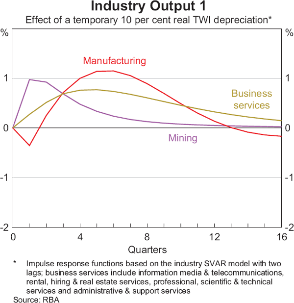
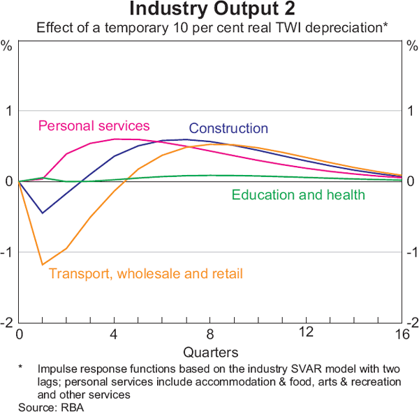
After about one year, output in most sectors is higher than prior to the depreciation. This is likely to reflect two effects: the increase in export competitiveness and the reduction in competition from imports for trade-exposed industries, and the second-round effect of higher aggregate domestic demand due to higher employment and income from the positively affected industries. Consistent with these effects, the two most trade-exposed industries – manufacturing and mining – experience the larger and more rapid increases in output; a 10 per cent exchange rate depreciation causes output in these industries to be higher by around 1 per cent after ½–1½ years. The large effect on mining is somewhat at odds with large capital costs and long investment times typical for this industry, which would suggest that supply in this industry would not typically respond quickly. Rather, the estimated effect may imply that it is possible to work the existing capital a little harder when output prices are higher, but not for a long time; this could also explain why the estimated effect is short lived compared with other industries. The effect on business services is also substantial, which may be due to the flow-on effect from the higher activity in other industries such as manufacturing and mining, given that the trade exposure of business services is not very high. Output for most other service industries increases to a smaller extent, which may reflect their lower exposure to trade. While the construction industry is subject to very little export demand or import competition, construction output tends to be highly cyclical, and the exchange rate effect, which is similar to that of most services, could reflect strong second-round effects of the impact of the depreciation on overall economic activity.
For a number of sectors, the estimates suggest that an exchange rate depreciation causes output to decrease in the first few quarters. For industries more directly exposed to household spending, such as retail services, this could reflect the initially negative effect on spending resulting from the higher cost of imports. Moreover, while retail and wholesale trade have a low share of imported inputs in the production of the distribution service, the demand for this service is linked to the cost of the good sold, which accounts for about half of the final price of the good. Since a large share of retail goods is imported, their cost varies with the exchange rate and so activity associated with their distribution is also likely to vary with the exchange rate. Beyond the effect on household spending, an exchange rate depreciation may also have a negative effect on firms' profits, owing to the increased cost of imported investment goods and intermediate inputs. This could explain the initially negative effect on manufacturing, which – as noted above – has a comparatively high share of imported inputs. The large initial negative effect on the transport, wholesale and retail sector could also be partly due to the initial profit effect, since imported inputs in the transport industry largely consist of fuel, where prices adjust very quickly, and in full, to exchange rate changes. Of course, similar to the estimates of the effect of the exchange rate on aggregate output, the estimates of the industry effects are subject to large confidence intervals and so a number of these effects may not be statistically significantly different from zero.
The Exchange Rate and Inflation
Exchange rate movements also affect consumer price inflation, directly through their effect on prices of imported consumer goods and indirectly through the cost of imported goods used in production and the increased demand for domestic goods. The effect of exchange rate movements on inflation has been discussed in detail in a previous Bulletin article (Chung, Kohler and Lewis 2011). These results are summarised in Table 3, together with the estimates from the SVAR and DSGE models.
| Total effect on price level |
Peak effect on year-ended inflation |
Peak timing |
|
|---|---|---|---|
| Model | Per cent | Per cent | Quarters after depreciation |
| Mark-up model | 1.1 | 0.4 | 9 |
| Phillips curve | 0.8 | 0.3 | 8 |
| SVAR | 1.7(b) | 0.7(b) | 12(b) |
| DSGE | 1.0(b) | 0.5 | 4 |
|
(a) Inflation refers to trimmed mean inflation; peak timing refers to effect on year-ended
inflation; SVAR results are from two-lag model Source: RBA |
|||
For most models, a permanent depreciation of 10 per cent leads to an increase in year-ended trimmed mean inflation of around ¼–½ percentage point over each of the following two to three years.
Conclusion
This article reviews estimates of the effect of real exchange rate changes on Australian output. The range of models analysed suggests that a temporary 10 per cent depreciation of the exchange rate increases the level of GDP temporarily by ¼–½ per cent over one to two years; a permanent 10 per cent real depreciation is estimated to increase the level of GDP by around 1 per cent after two to three years. Year-ended inflation is estimated to be higher by ¼ to ½ percentage point in the two to three years following a permanent 10 per cent depreciation.
At an industry level, unsurprisingly, output in the trade-exposed mining and manufacturing industries is most affected, as well as in business services, which often benefit from activity in these industries. It should be noted, however, that such estimates are subject to significant uncertainty. Moreover, for any given episode of exchange rate depreciation (or appreciation), output is also likely to react to other concurrent macroeconomic factors, including those that may have triggered the exchange rate depreciation, such as a change in the terms of trade.
Appendix A
This article reports estimates from a number of models used at the Bank that allow analysis of the impact of exchange rate movements on activity and inflation.
SVAR
The structural vector auto regression (SVAR) model is based on work by Lawson and Rees (2008). An updated and modified version (which underlies the estimates in this article) is in Manalo, Perera and Rees (forthcoming). The model is estimated with data from 1985:Q1 to 2013:Q2.
The aggregate model includes Australian and US GDP (deviations from trend), the terms of trade, trimmed mean inflation, the cash rate and the real TWI. Note that this model relates the level of the exchange rate to the inflation rate – not to the price level, as in the single equation models in Chung et al (2011) – and so changes in the exchange rate relate to changes in the inflation rate. Because of this specification, changes in the exchange rate can appear to have permanent effects on the inflation rate.
Each industry model is estimated separately, and includes industry output (deviation from trend) in addition to the variables included in the aggregate model. The sum of the estimates from each industry model, weighted by industry shares, suggests a very similar profile to the aggregate SVAR for the results considered here, even though those models are estimated separately. The size of the estimated model responses differ somewhat between a specification including two lags and three lags, but it is difficult to select a preferred specification out of these two options.
In this type of model, a change in the exchange rate is usually modelled as a temporary shock to the exchange rate. All variables in the model (including the exchange rate itself ) are allowed to respond endogenously, except for the cash rate, which is held constant for the estimates presented here. The model responses return to their starting point after some time, so the exchange rate endogenously (and gradually) returns to its baseline level after the initial shock. A permanent shock is modelled as a sequence of temporary shocks, which (together with the lagged responses of the exchange rate to the preceding shocks) force the exchange rate to remain at the higher level for the period analysed.
DSGE
The dynamic stochastic general equilibrium (DSGE) model is based on the model in Jääskelä and Nimark (2011). The model is estimated with data from 1993:Q1 to 2013:Q2.
The model includes Australian GDP, household consumption, private investment, government expenditure, exports, imports, trimmed mean inflation, the real exchange rate and hours worked. Foreign variables are major trading partner GDP, G3 interest rates and G7 inflation. As with the SVAR model, the exchange rate relates to inflation and so changes in the exchange rate relate to changes in the inflation rate (rather than the price level).
Again, this model naturally allows for temporary shocks in the exchange rate, with the model estimates (including the exchange rate) returning to the steady state after some time. The cash rate is not held constant for the estimates presented here. A permanent shock is implemented as a sequence of shocks that holds the exchange rate at the desired level for two years, before allowing it to revert endogenously to its baseline value.
Export and import equations
A third approach simply models the expenditure-switching effect on exports and imports, and then scales the export and import effects according to their share of GDP. This approach does not take account of additional effects on GDP arising from a change in domestic demand. Single equation models do not take explicit account of feedback from the dependent variable to independent variables, or feedback within the independent variables. They are also more suited to an analysis of permanent, rather than temporary, changes to an independent variable.
Exports are modelled with separate equations (error-correction models) for manufactures and services exports. In line with previous literature, resource exports are assumed to not be sensitive to changes in the exchange rate in the short to medium term, owing to the large capital costs and long investment times typical for this industry. For a few quarters, it may be possible to lift production by working the existing capital a little harder, but this cannot usually be kept up for longer periods without installing new capital. For manufactures exports, the model is as follows:
In words, manufactures export volumes (man, in logs) are modelled as a function of their own lags; major trading partner GDP (mtp, in logs); the real exchange rate (rer, export weighted, in logs); the effective rate of assistance (era); and an error term ∈t. The equation is estimated from 1985:Q1 to 2013:Q3.
A 10 per cent depreciation increases manufactures export volumes by 5 per cent overall and the effect is comparatively fast, with most of this complete within two years. Since manufactures exports comprise 2 per cent of GDP, this would increase GDP by 0.1 per cent. For service exports, the model is as follows:
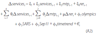
Service exports (services, in logs) are a function of their own lags; major trading partner GDP (mtp, in logs); the real exchange rate (rer, in logs, export weighted); and an error term. Olympics is a variable that takes the value of one in 2000:Q3 (the date of the Sydney Olympics) and the value of minus one in 2000:Q4 (and zero otherwise); SARS and Sep11 are dummies that are one in 2003:Q2 and 2001:Q4, respectively, and zero otherwise; and timetrend is a time trend. The equation is estimated from 1991:Q1 to 2013:Q3.
A 10 per cent depreciation increases service export volumes by 13 per cent overall, but the effect is quite slow and after two years service exports have increased by around 8 per cent. Service sector exports are 3 per cent of GDP, resulting in an increase of GDP by 0.2 per cent after two years. For imports, the model is as follows:
Import volumes (import, in logs) are modelled as a function of their own lags; domestic demand (measured as final consumption expenditure plus gross fixed capital formation minus ownership transfer costs) plus exports (dom, in logs); the relative price of imports to the price of domestically produced and consumed goods (measured by the implied deflators of imports and of GDP minus exports) (relprice, in logs); the cash rate (cashrate, in logs); inventories; and an error term, ∈t. The equation is estimated from 1987:Q2 to 2013:Q3. The exchange rate affects imports through the relative price of import goods, which has a long-run coefficient of −0.55. The import price equation is specified as in Chung et al (2011), which yields a long-run coefficient for exchange rate changes of 0.8.
A 10 per cent depreciation increases import prices by 8 per cent, which in turn decreases imports by 4.4 per cent. Imports have a share of 20.1 per cent of GDP, yielding an addition to GDP of 0.9 per cent. Most of this is passed through after two years.
Mark-up model and Phillips curve
These single equation models for inflation are based on those discussed in Chung et al (2011), derived from an import price model and then a model that relates import prices to consumer prices. The models are estimated using data from 1990:Q1 to 2013:Q2. As mentioned above, single equation models are less well suited to capture some second-round effects and are also better suited to an analysis of permanent shocks, rather than temporary shocks.
Footnotes
The authors are from Economic Analysis Department. They would like to thank Daniel Rees and Hao Wang for help with some of the model estimates. [*]
These ‘expenditure-switching’ channels are the most obvious ways in which a depreciation (or appreciation) affects real activity. There are other channels through which real activity can be affected, such as through higher real debt burdens of unhedged debt denominated in foreign currency, or the impact on capital flows if the relative attractiveness of domestic and foreign investment is affected by the depreciation (see, for example, Mark (2001) or Montiel (2009) for more detail). [1]
Agriculture, forestry & fishing, electricity, gas, water & waste and public administration & safety have been excluded from this analysis, because activity in those sectors is significantly influenced by supply-side developments. Financial & insurance services, which were estimated to experience a protracted negative effect from a depreciation, are not discussed in the results presented here. The result for this sector is difficult to explain, and may be a consequence of difficulties in modelling activity in this industry. [2]
References
Chung E, M Kohler and C Lewis (2011), ‘The Exchange Rate and Consumer Prices’, RBA Bulletin, September, pp 9–16 .
Jääskelä J and K Nimark (2011), ‘A Medium-scale New Keynesian Open Economy Model of Australia’, Economic Record, 87(276), pp 11–36.
Lawson J and D Rees (2008), ‘A Sectoral Model of the Australian Economy’, RBA Research Discussion Paper No 2008-01.
Manalo J, D Perera and D Rees (forthcoming), ‘Exchange Rate Movements and the Australian Economy’, RBA Research Discussion Paper.
Mark NC (2001), International Macroeconomics and Finance: Theory and Econometric Methods, Blackwell Publishers Inc, Malden, Massachusetts.
Montiel PJ (2009), International Macroeconomics, Wiley-Blackwell, Malden, Massachusetts.

