It’s a pleasure and honour to be addressing the Australian Conference of Economists and to have the opportunity to connect with so many professional colleagues and friends. Thank you to Bob Breunig and the rest of the organising committee for the invitation. Before I start, I would like to acknowledge the Traditional Owners of this land, the Ngunnawal people, and the other First Nations people who are custodians of this part of our beautiful country. We are very lucky in Australia to have a First Nations people that take such good care of our land and culture and pass this on to future generations. I pay my respect to elders past and present and extend this respect to any First Nations people here with us today.

The RBA is mandated to maintain, on average over the medium term, a 2–3 per cent band for inflation and sustained full employment – that is, the current maximum level of employment that is consistent with low and stable inflation. The target outcome is therefore clear, ensuring inflation returns sustainably to target. To do this, we have to account for a myriad of different economic forces that influence the productive capacity of the economy, aggregate demand, and costs and inflation.

To bring all of these factors together, it’s helpful to take a simplified top-down view. Figure 1 does this by representing the two parts of our mandate. The vertical axis represents inflation, with a dashed line at 2.5 per cent, which is the midpoint of the target band. The horizontal axis represents conditions in the labour market and the economy more broadly; on the right-hand side of the vertical line there is spare capacity in the economy, and the labour market is operating below full employment. On the left-hand side, the economy is operating beyond its sustainable capacity, and the labour market is tight.

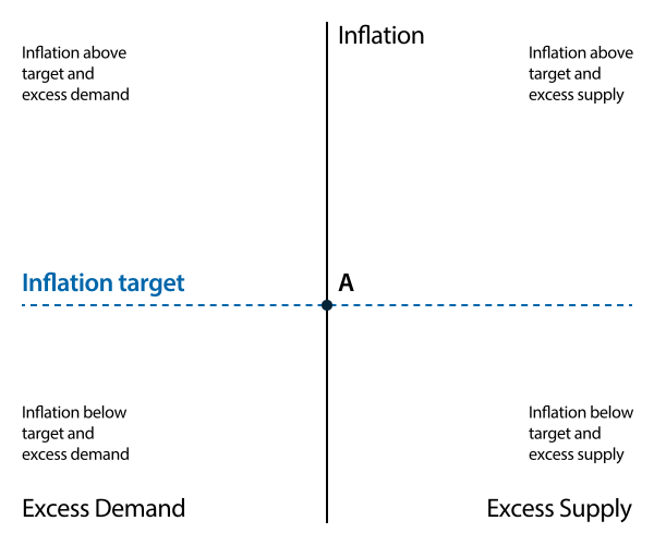
In Figure 1, from any given starting point, if a central bank lowers interest rates, the economy will move to the left and up. This is because lower interest rates tend to increase demand without affecting supply (resulting in a leftward shift) and thereby also increase inflationary pressure (an upward shift) and conversely, if rates are raised, the economy will move to the right and down.

This reflects the fact that monetary policy is a demand management tool. We can’t use it to materially change the economy’s trend rate of productivity growth or maximum sustainable employment, and as a small open economy we are buffeted by changes in the global environment.

Why is it important to highlight this? As the Governor discussed last year, over the long run our two objectives go hand in hand and there is no trade-off. Low and stable inflation also supports sustainable growth as it allows households and businesses to plan and invest without worrying about inflation.¹ But ultimately, structural drivers like demographics and productivity determine trend growth, and these trends don’t typically vary enough to drive short-run cycles.

So, what does drive the short-run cycles we see? We typically conceptually put the drivers into two buckets – demand shocks and supply shocks – though recently it has often been the case that a shock or event affects both demand and supply simultaneously; the COVID-19 pandemic is a vivid recent example.

In the case of demand shocks, inflation and the labour market will broadly move in the same direction relative to our mandate. Starting from a balanced position with inflation at target (point A in Figure 1), if demand picks up – for example, due to a lift in confidence and so spending – the economy will start operating above its sustainable capacity. This then creates inflationary pressures, putting us in the top-left quadrant. Monetary policy can be used to slow demand and so economic activity and inflationary pressures, bringing the economy back into balance over time.

But some types of economic disturbances, or shocks, will put our mandate outcomes into conflict by pushing up inflation while also weighing on demand and activity – putting us in the top-right quadrant. These will often be shocks that temporarily push up some costs or prices, which simultaneously lifts inflation but dampens demand as households and businesses have to bear these higher costs. These shocks can have a broad impact across many parts of the economy, such as the recent conflict in the Middle East that has lifted global energy and related prices, or they can be narrow and short-lived such as the sharp temporary increase in banana prices we experienced in 2006 after Cyclone Larry.

In short, supply or relative price shocks can create a trade-off for monetary policymakers if they are likely to have a persistent impact on inflation and the broader economy. All else equal, a persistently higher outlook for inflation suggests that interest rates should be raised. But at the same time, weaker economic activity and so more excess supply suggests that interest rates should be cut, all other things equal.

This trade-off cannot be avoided. A central bank can only decide how to balance the impact on inflation and activity, while ensuring that temporary shocks do not become persistent inflation.

In the years leading up to the COVID-19 pandemic, these types of adverse supply shocks had become rarer, compared with the 1970s and 1980s. Economic outcomes in Australia and globally had been driven more by a number of long-term structural drivers, like slowing productivity growth and the disinflationary impact of the expansion of China’s manufacturing sector, or factors that influenced aggregate demand, like confidence or overseas financial sector disruptions.

But more recently, these sharp adverse supply shocks have become more frequent, meaning the Monetary Policy Board and the RBA have had to navigate the policy trade-offs repeatedly. And we could see this continue going forward; economic spillovers from rising geopolitical tensions, trade fragmentation, and the increasing prevalence of extreme climate events are just some of the shocks we are now experiencing. While these trends will also cause longer-run structural shifts in the global economy (including Australia), as we have seen in recent years, they can also lead to sharp economic disruptions in the here and now.

So, against this background, today I am going to talk in a bit more detail about how these different factors – longer-term structural shifts in supply, demand and short-term supply shocks – play through the economy and influence a central bank’s choices. In doing so, I will give particular focus to short-term adverse supply shocks, the trade-offs they create, and what it might mean for policy trade-offs if these types of shocks occur more often.

Before I start though, I wanted to recognise that this topic of trade-offs is one that we have been discussing a lot lately in speeches and other communications and is a very active area of research and analysis for the RBA. This reflects how important we feel it is – not only for us as policymakers, but also for the broader public – to understand the nature of these trade-offs and what they mean for monetary policy, both in the current environment and into the future.

A framework for macro trends and shocks

For this speech I am going to split the economic shocks and shifts that a central bank has to navigate in setting monetary policy into three buckets: slow-moving structural drivers of supply capacity; shorter-term cyclical drivers of demand and activity, which push inflation and activity in the same direction; and shorter-term cost or supply shocks, which push current inflation and activity in opposite directions.

This is obviously a simplification. Deciding what is cyclical and what is structural is not a simple, bright-line distinction. And many shorter-term economic disturbances have elements of demand and supply: empirical research by the RBA has shown that it can be difficult to separate the two even with the benefit of hindsight.² This can reflect the complex nature of the shock. For example, the COVID-19 pandemic and the resulting policy response affected demand as well as the economy’s supply capacity (in other words, lockdowns). In some cases, a factor or event can have both a cyclical and structural impact, as it propagates through a complex and interconnected economy.

For the purpose of this speech, splitting into these three buckets is a useful conceptual simplification. But it’s very important to keep in mind that the real world is not so neat and tidy, and policymakers have to continuously navigate through this messiness.

Slow-moving trend changes

In order to assess the extent of capacity pressures now and in the future, central banks need to understand slow-moving structural changes in potential supply. These determine the productive capacity of the economy, and therefore ultimately what rate of growth in activity and conditions in the labour market are sustainable. In other words, we need to have a sense of the pace of trend growth to judge whether GDP is growing ‘quickly’ or ‘slowly’ relative to that trend.

As I noted before, and have discussed in other speeches, monetary policy can’t significantly influence productivity and potential output over the medium term.³ Rather, trend productive capacity is influenced by a myriad of other factors that influence the trends in the three Ps: productivity, participation and population.

Many argue that one of the key causes of global inflation during the 1970s, apart from increases in oil prices, was a mis-assessment of underlying sustainable economic capacity, with policymakers thinking economies could grow faster than what proved to be their actual underlying trend.⁴ As such, we invest a lot in trying to understand the long-run drivers of economic growth.⁵

Still, changes in these trends don’t tend to create sizeable short-term trade-offs for monetary policy between inflation and activity for two reasons. First, given the structural nature of many of these drivers, they tend to be slow moving and have more limited impacts year-to-year. For example, the slowdown in productivity growth we have seen over recent decades has had a notable impact on potential, but the effects have been relatively gradual (Graph 1).

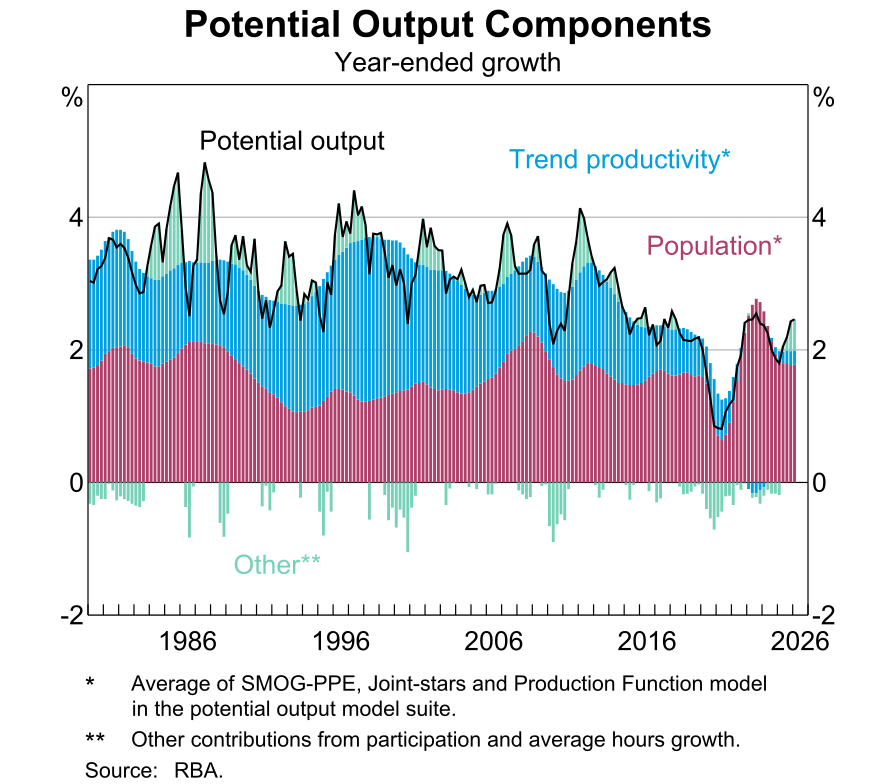
Second, these changes represent a shift in the productive capacity of the economy and so don’t necessarily create a trade-off between our objectives. If growth in potential supply slows, monetary policy can help to guide activity into line with the new path for potential output without necessarily creating a challenge for the inflation target.

What it can’t do is keep us on the previous trend path with low and stable inflation. So, there is no trade-off here for policy. In fact, in many cases the adjustment to the new trend path may happen naturally – people may realise growth is going to be faster or slower in the future and adjust their behaviour ahead of time. This is exactly the assumption we made in lowering our medium-term productivity forecasts in mid-2025.⁶ Graph 2 shows these dynamics well, across a number of countries, households have adjusted to lower prospective growth in activity and income as productivity growth has slowed, by reducing consumption to match the outlook for income.

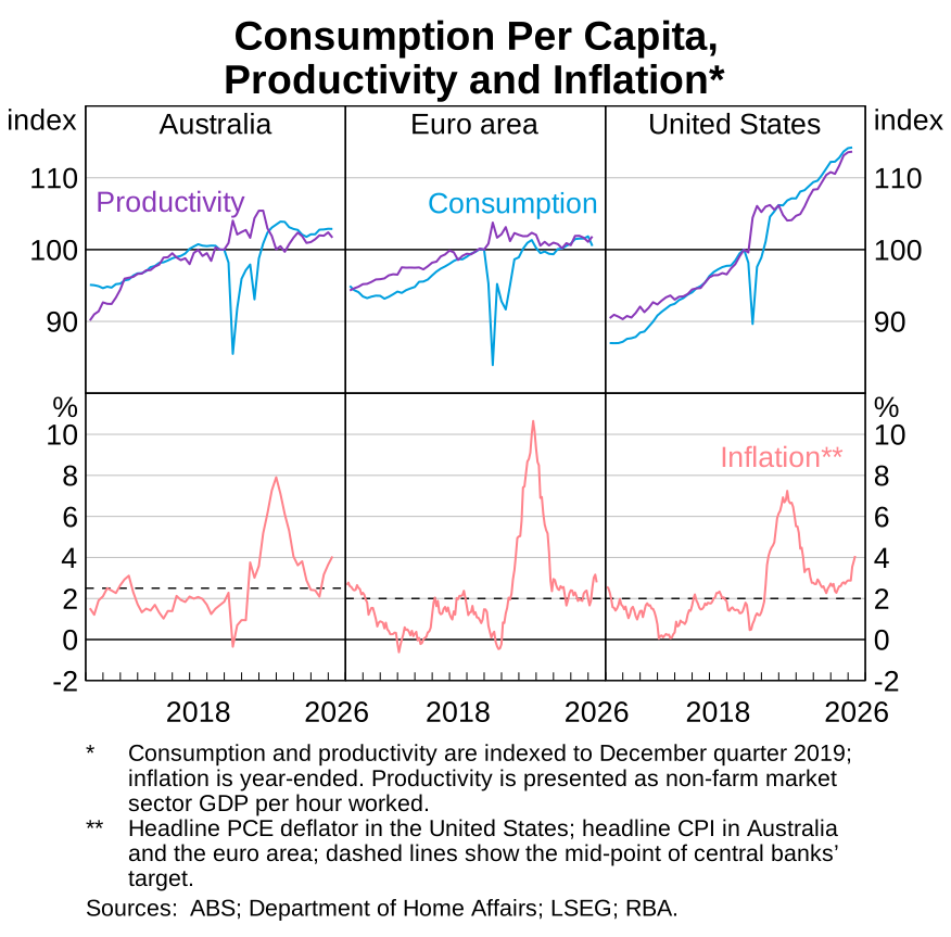
The analysis above clearly highlights the importance of identifying shifts in these trends. It also highlights that doing this in real time is difficult. To tackle this, we continuously review our assessment and judgement about underlying trend growth.

As part of this ongoing reassessment, there are several factors that are going to be important in driving potential output growth. One is the outlook for population growth and labour force participation. Another is AI, which has the potential to significantly lift productivity growth over the medium term, though the precise scale and timing of any such effect is highly uncertain. And a third is climate change, which has the potential to significantly impact productive capacity over the short and long run – for example, by changing the yield of farmland, the effectiveness of workers, or through natural disasters.

Demand shocks

The second set of economic drivers I want to talk about are shorter-term shifts in aggregate demand – demand shocks. A natural example is a change in confidence, which influences how much people want to spend versus save today.

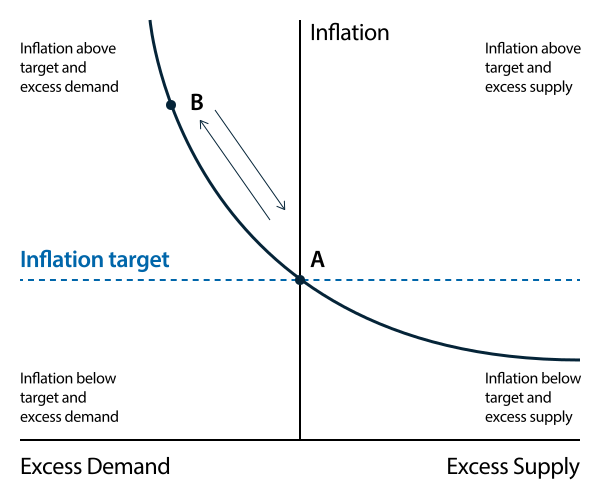
We can analyse these dynamics using a Phillips curve, which traces out the relationship between inflation and measures of spare capacity, and which I and the Deputy Governor have discussed extensively in our recent speeches.⁷ For an economy that starts out at balance (point A in Figure 2), an exogenous increase in demand and activity pushes the economy to be operating above its sustainable productive capacity and also pushes inflation above target (i.e. the economy moves to point B). Monetary policy can respond to this, by raising interest rates to tighten financial conditions (so that they are restrictive), which works to bring the economy back into balance and return inflation to target.

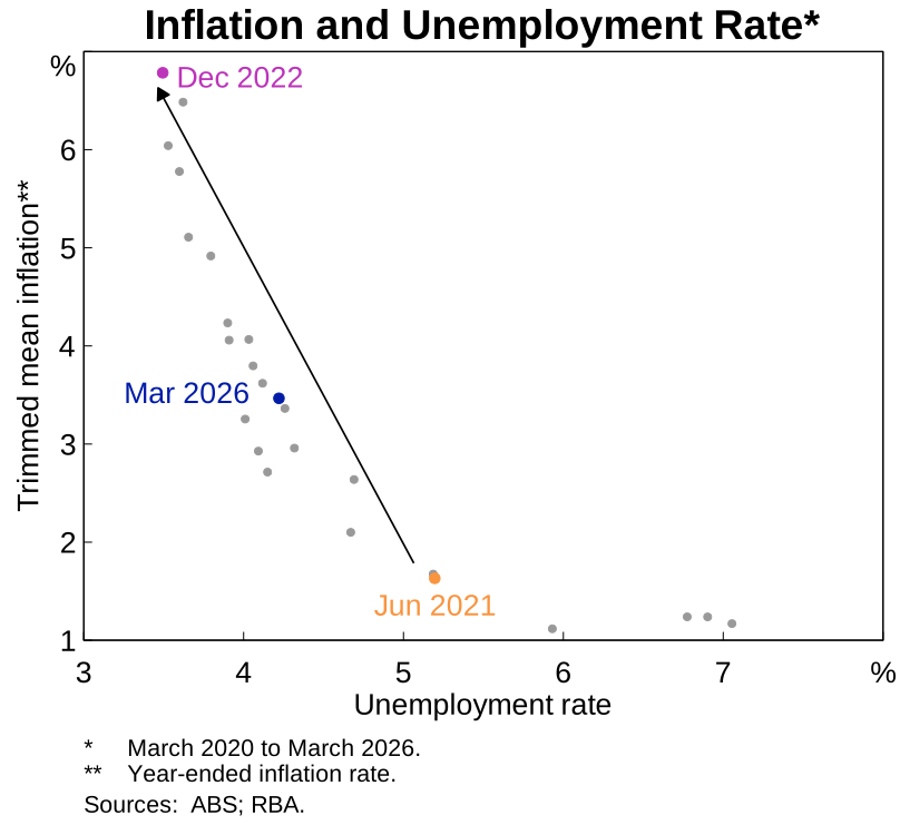
To make this more concrete, Graph 3 shows an empirical version of this relationship highlighting the post-COVID-19 experience. Coming out of the pandemic, unemployment fell to very low levels (and our quantitative estimates suggest that the economy was operating above its sustainable capacity), which contributed to a sharp pick-up in inflation. But as the economy has moved back towards balance, alongside some abatement in supply chain disruption and global inflationary pressures, inflation fell back towards the target range.

I want to be clear that I have significantly simplified this discussion. There is growing literature showing how these dynamics can become a lot more complicated when there are multiple sectors, supply chains and firms resetting prices at different rates, especially if demand shifts across sectors.⁸ The post-COVID-19 period is a perfect example. They can also become more complicated because different households could be differentially exposed to monetary policy and the underlying demand shock.⁹ Still, in general, the point remains that demand shocks will tend to push economic activity and employment, and inflation in the same direction, meaning fewer trade-offs for policy.

Supply (relative price) shocks

The third bucket of developments I want to talk about are ones that temporarily push inflation and activity in different directions. These naturally create a trade-off for monetary policy and the economy.

These shocks can be thought of as a shift up and potentially a steepening of the Phillips curve: for any given level of domestic economic activity (typically captured as the unemployment rate), inflation will be higher (Figure 3). Even if aggregate demand and the economy’s productive capacity are in line with each other, inflation will be too high (C). For inflation to be at target while the shock is putting upward pressure on costs, there would need to be some excess capacity (D).

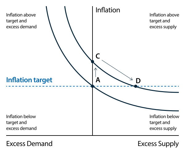
This changes the set of available choices for monetary policy while the shock is propagating across the economy – we can have inflation closer to target, or the economy operating closer to capacity (the labour market at full employment), but we can’t have both.

What are these types of shocks? Well, many of them will be relative price shocks where the price of a single good or specific set of goods goes up. In some cases, this will be an intermediate input, such as the recent increase in oil and related commodity prices. These shocks can also appear in consumer prices – for example, the increase in the price of imported medical equipment during the COVID-19 pandemic, when global demand increased and supply couldn’t fully respond. These shocks could also be positive in the sense that they push inflation down and activity up temporarily – for example, a bumper harvest that reduces some grocery prices.

We can see exactly this type of dynamic in Graph 4, which shows the empirical Phillips curve, but includes points capturing our current forecasts from June 2026 onwards. The current oil price shock has shifted the curve out somewhat, implying higher underlying inflation for any level of unemployment (Graph 4).

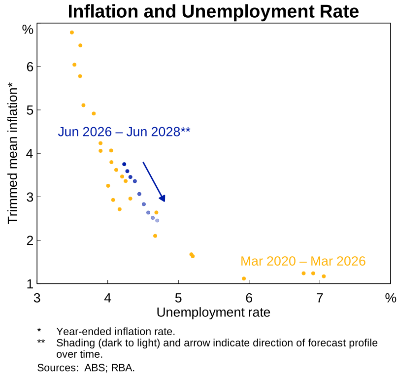
These shocks have direct effects, pushing up the price of the good itself. But they can also have second-round effects, putting upward pressure on the prices of other goods. This is likely to be the case when they are intermediate goods (such as oil). These shocks can also potentially shift inflation expectations and therefore other pricing and wage decisions. While monetary policy can’t undo the initial shock, it can potentially limit the indirect and second round effects, thereby limiting how far the Phillips curve shifts.

Ultimately, though, some economic costs are unavoidable. All policymakers can do is strike a balance in the face of a worsening trade-off.

What determines the extent of the trade-off?

For the rest of the speech, I am going to focus on these temporary supply, or relative price shocks. I want to discuss in a little bit more detail some of the factors that influence the extent of the policy trade-off they create for a central bank. I’ll also focus on how some of these might change in a world where we face more frequent supply shocks.

To start off, I thought it would be worth highlighting the oft-cited policy prescription for temporary supply shocks – which is to ‘look through’ them, allowing inflation to rise temporarily before falling back to target with limited monetary policy response.¹⁰ This approach is only appropriate if policymakers are confident that the shock will not be persistent, that second-round effects will be limited and that inflation expectations will remain anchored.

Persistence and second round effects

The prevailing wisdom to look through short-term supply or relative price shocks is predicated on the idea that the shock and its impacts are thought likely to be quite short-lived. So, while the price of say, oil or bananas, will rise, they will either fall back down quickly, or represent a one-off increase in the price level of that good, with little ongoing effect on inflation.

This assumption is important for two reasons. First, if people expect the shock to be over quickly, they are less likely to respond to it. For example, businesses may be less likely to raise their prices in response to higher costs, knowing they will lower them again soon as costs fall. And households may be more willing and able to just smooth through temporary hits to their spending power, rather than cutting back on consumption. So, the effect on inflation and activity will be more limited.

Second, monetary policy only affects the economy with a lag. So, if the shock is short-lived, the inflationary impact will have abated by the time monetary policy starts having an influence on the economy.

By contrast, if the shock is expected to be more persistent, it is likely to have larger impacts and create greater risks of inflation expectations shifting. And policy may come into play while the shock is still influencing inflation. In this world, it may not be right for monetary policy to ‘look through’.

The nature of the underlying shock is also important. If the shock hits only a small number of items, which aren’t inputs into other goods, its impacts may be narrower and shorter-lived. But if it flows into complex supply chains, the initial cost increase could trickle through the economy over time, creating more drawn out and widespread inflationary pressure.¹¹ And similarly, the starting point for the economy matters. When the economy is operating beyond its sustainable capacity, underlying inflation is above-target and we are on a steep part of the Phillips curve, firms may be more likely to pass on changes in their costs.¹²

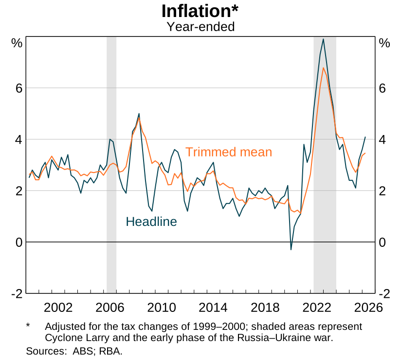
We can see these differing dynamics in two contrasting examples from history (Graph 5).

One is Cyclone Larry in 2006. This cyclone in Far North Queensland damaged a large amount of agricultural land, including a very large share of the banana crop. This caused banana prices to rise by around 400 per cent, pushing up headline inflation by ¾ percentage point. However, this quickly unwound and had no spillovers to other prices. Notably, this caused a sharp divergence between headline inflation, which spiked, and underlying inflation, which abstracted from the sharp move in banana prices. Monetary policy settings were not changed in response, and the RBA was clear that underlying inflation would not be impacted; this demonstrates the value of analytical measures of inflation like trimmed-mean, which tend to be a better predictor of headline inflation one-to-two years out.¹³

The post-COVID-19 inflation shock was quite different. While initially the expectation was that it would be temporary, in practice imbalances in global supply and demand stemming from COVID-19-related disruptions to supply chains, shipping congestion, shifts in consumption patterns (as well as much stronger-than-expected demand, including as a result of expansionary macroeconomic policy) and the ongoing conflict in Ukraine led to more sustained and broad inflationary pressure.¹⁴ As a result, central banks around the world had to respond with tighter policy.

Expectations

As I noted earlier, another key assumption in the recommendation to ‘look through’ supply shocks is that inflation expectations don’t pick up in response to the higher inflation, at least not meaningfully. As discussed in recent speeches, if they do this, it can lead to larger and potentially more persistent increases in inflation, as the Phillips curve effectively shifts up by more or for longer, shifting the trade-offs faced by policy.

But why are inflation expectations such a key focus of central banks currently when, at least in developed countries, inflation expectations (particularly longer-run expectations) appear to have been anchored for decades?

A key reason why central banks remain focused on inflation expectations is that how central banks respond, or people expect them to respond, will tend to shape expectations. If people expect the RBA to do what is necessary to keep inflation contained, inflation expectations are less likely to rise and so actual prices to change. Put another way, it’s the Board’s credible focus on achieving the inflation target that helps keep expectations anchored and minimises the risk of persistent inflation.

Survey data on firms’ future pricing intentions is consistent with this intuition. For the April Macquarie BOSS Survey, we worked with the organisers to include a question asking businesses: ‘if the Iran conflict raised your costs by 10 per cent, how much would you pass on into prices?’. The average firm said 30 per cent. But for those firms that were very uncertain that the RBA would hit its target in the long run, they said 40 per cent. Similarly, ongoing work by RBA researchers has also highlighted how RBA actions and communication can shape the market perceptions of how the RBA will respond to shocks.¹⁵

And even if people’s expectations are anchored in the long run, their shorter-run expectations could still move. This is a place where the RBA has been investing in our understanding. Some research we put out last year highlighted how actual inflation outcomes can shape households’ short-run inflation expectations.¹⁶ When people have these backward-looking expectations, looking through supply shocks might be less optimal, as we may need some period of low inflation and higher unemployment to bring expectations back down if they start drifting up.¹⁷

Activity impacts

So far, I have focused on the inflation side of the trade-off, but obviously the other side of the coin is what happens to economic activity.

Older economic models tended to assume that temporary supply shocks had only small effects on overall economic activity, and in particular on the amount of excess capacity in the economy. This was especially the case when such shocks were confined to a single sector or a small number of products. However, a growing body of recent work highlights that sector-specific supply shocks can have spillover effects on activity and demand across the broader economy.¹⁸

As we have seen recently, large economic shocks can create uncertainty, reduce confidence and, for some, constrain spending on other goods and services.¹⁹ In turn, this can dampen household spending, and prompt firms to put investment decisions on hold and reconsider their hiring plans. These channels have been a key focus in recent weeks, particularly given the recent fall in consumer and business confidence. But thus far there are few signs of a marked slowdown in activity.

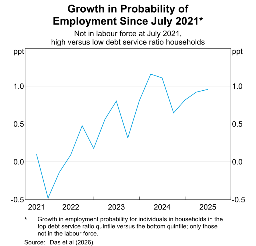
Another way households may respond if they are constrained is by trying to work more to increase their income. Recent joint RBA–IMF research found evidence of this, showing households responded to cost-of-living pressures in post-COVID-19 by increasing their labour supply. Those with a larger mortgage (all other things equal) who were more exposed to rising rates were more likely to enter employment (Graph 6). Such dynamics would help offset the initial negative supply shock, supporting economic potential and thereby at least partially offsetting inflationary pressure. Ongoing investments in data and research are allowing us to better understand these channels of shock transmission, including by building models that take constraints and household heterogeneity seriously.

What does this mean for monetary policy choices?

So, what does this discussion mean for how a central bank would respond to one of these shocks? To think about this, we can return to the stylised diagram from before. Ultimately when we are in the top-left or bottom-right quadrant in Figure 1, adjusting interest rates will bring both inflation back towards target and the economy back towards balance. But when temporary supply shocks push us into the top-right quadrant or bottom-left quadrant, policy will face a trade-off between having inflation close to target and keeping the economy close to its maximum sustainable level for activity and employment.

Ultimately, if some persistent inflationary pressure is expected, monetary policy may need to be tightened. But by how much depends on all the factors I have discussed so far and the trade-offs they create.

To illustrate this, it is helpful to return to the earlier stylised Phillips curve from Figure 3 and focus in on the top-right quadrant, considering the different outcomes we could arrive at and the paths that might lead us there (Figure 4). If the economy is hit by a supply shock that has a persistent upward effect on inflation, with the economy ending up at a point like E, with underlying inflation well above target, some tightening might be called for.

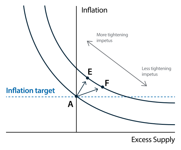
But monetary policymakers would have to weigh this against the softening of economic activity and the labour market. If activity were to be more negatively affected by the shock (point F), the bias towards tightening might be more limited.

It’s worth keeping in mind that this discussion is very simplified, and actual policy would take into account a large number of factors, including how costly the central bank thought inflation was, relative to unemployment, and the dynamics and transmission of policy through the economy.

And to reiterate an earlier point, in practice, policymakers don’t know the exact nature of the shocks hitting the economy and the extent of excess supply, so things aren’t as simple as they appear in Figure 4. And as I have discussed throughout, our actions can actually influence the trade-offs themselves and where the Phillips curve ends up, by influencing expectations. In short, there’s a lot to consider.

How might this change in a world with more frequent shocks? Several factors could intensify the trade-offs. Inflation may respond more strongly if shocks occur while underlying inflation is already elevated – reflecting firm pricing behaviour or an increased risk of inflation expectations becoming de-anchored.

At the same time, the effects on activity could be larger if households and businesses become more cautious or if their financial buffers have been eroded by earlier shocks, although this may be partly offset if households increase labour supply.

Ultimately, while supply shocks create difficult trade-offs, they do not lessen the importance of maintaining low and stable inflation. The Board will continue to act as needed to ensure inflation returns to target and the labour market to sustainable full employment.

Investing in knowledge and capability

As I have highlighted, supply shocks create unavoidable trade-offs for a central bank and the broader economy, and these trade-offs are complex and multifaceted. What has changed is that these shocks appear to be becoming more frequent. That means the RBA – and the economy more broadly – may have to face these trade-offs, and the costs that come with them, more often in the years ahead. That makes it even more important that we understand these shocks well, prepare for them, and respond in a way that minimises the risk of persistent inflation while supporting sustainable activity.

To help us navigate through these complexities, the RBA is investing in our knowledge, people and frameworks. Both the Deputy Governor and I have discussed some of the work in this space in our recent speeches. This includes research and investment in new models and capability. This ongoing work is also captured in the RBA’s monetary policy research agenda, which was recently published on our website;²⁰ we intend to use it to both guide our research and increase our engagement with research economists.

At the same time, we have launched a number of new initiatives to increase our engagement with the economics and policy community. These are aimed at strengthening our ties to academia, think tanks and the broader economic community to help us test our thinking, and bring in new cutting-edge knowledge and capabilities. Relatedly, we have recently launched Insights: An RBA Staff Series, a new publication that provides a platform for RBA staff to publish analytical notes on topics relevant to our remit.²¹ These pieces, many of which will be prepared by my incredible team, are shorter than some of our more detailed research publications and, in contrast to our official ‘Bank-view’ publications like the Bulletin, they expressly reflect the authors’ views. At times, this means they could put forward alternative views and perspectives, which is a normal and essential part of good research and analysis practice and robust challenge.

And while it is important that the public hears regularly from the RBA’s senior leaders, and more recently from members of the Monetary Policy Board, we are also looking to broaden how we communicate and make more of the RBA’s analysis accessible to a broader audience. This includes creating more opportunities to share staff analysis directly, strengthening transparency and contributing to the economic conversation.

Additionally, the RBA’s 2026 Annual Conference will focus on the topic of trade-offs. It will bring world-leading academics and policymakers to the RBA to discuss these issues, which can help us continue to build our knowledge and frameworks.²² I and my colleagues are very much looking forward to discussing these issues now and into the future.

Endnotes

* I would like to acknowledge and thank Jonathan Hambur who substantially contributed to the drafting of this speech. I would also like to thank Alex Ballantyne, Anthony Brassil, Michele Bullock, Adam Cagliarini, Natasha Cassidy, Nicholas Dwyer, Samuel Evangelinos, Andrew Hauser, Suzanne Houweling, Chris Kent, Callum Ryan, Ekaterina Shabalina, Michelle Wright and Ada Zhu for their comments on the speech, and Jenny Lui for her assistance with the speech figures. Any errors or omissions are my own. For the data source from the Australian Bureau of Statistics PLIDA dataset, see PLIDA Disclaimer.

1 Bullock M (2025), ‘The RBA’s Dual Mandate – Inflation and Employment’, Speech at the Anika Foundation Fundraising Lunch, Sydney, 24 July.

2 Read M (2024), ‘Sign Restrictions and Supply-demand Decompositions of Inflation’, RBA Research Discussion Paper No 2024-04.

3 Some recent papers have argued that monetary policy can influence potential. For example, some have argued that expansionary monetary policy can disproportionately support industry leaders, helping to entrench market power (e.g. Liu E, A Mian and A Sufi (2022), ‘Low Interest Rates, Market Power and Productivity Growth’, Econometrica, 90(1), pp 193–221). However, evidence for Australia does not support this finding (e.g. Nolan G, J Hambur and P Vermeulen (2023), ‘Does Monetary Policy Affect Non-mining Business Investment in Australia? Evidence from BLADE’, RBA Research Discussion Paper No 2023-09). Similarly, some have argued that contractionary monetary policy can weigh on innovation, leading to medium-run declines in productivity (e.g. Moran P and A Queralto (2018), ‘Innovation, Productivity and Monetary Policy’, Journal of Monetary Economics, 93, pp 24–41). While there is some evidence of such a dynamic in Australia, it appears to be more short-lived and heterogenous, particularly once focusing on adoption of technologies not just innovation (e.g. O Majeed, J Hambur and R Breunig (2025), ‘Does Monetary Policy Impact Innovation? Evidence from Australian Administrative Data’, Journal of Macroeconomics, 86).

4 For example, Orphanides A (2003), ‘The Quest for Prosperity Without Inflation’, Journal of Monetary Economics, 50(3), pp 633–663.

5 For some overviews of this work, see Plumb M (2025), ‘Why Productivity Matters’, Speech at the Australian Business Economists Annual Forecasting Conference, Sydney, 27 February; Hunter S (2025), ‘Why Productivity Matters for Central Bankers’, Speech at the Citi Australia and New Zealand Investment Conference 2025, Sydney, 15 October.

6 RBA (2025), ‘Chapter 4: In Depth – Drivers and Implications of Lower Productivity Growth’, Statement on Monetary Policy, August.

7 The Phillips curve shown here assumes inflation expectations are anchored at the inflation target, meaning that when activity is in balance, inflation will be at target.

8 See, for example, Rubbo E, ‘Networks, Phillips Curves, and Monetary Policy’, Econometrica, 91(4), pp 1417–1455; Baqaee D and E Fahri (2022), ‘Supply and Demand in Disaggregated Keynesian Economies with an Application to the COVID-19 Crisis’, American Economic Review, 112(5), pp 1397–1436.

9 In the paper, Acharya S, E Challe and K Dogra (2023), ‘Optimal Monetary Policy According to HANK’, American Economic Review, 113(7), pp 1741–1782, the authors show that in such frameworks stabilising inflation and the output gap no longer remains ‘optimal’.

10 For instance, the Reserve Bank of New Zealand’s March 1990 Policy Targets Agreement (published in Reserve Bank Bulletin, 53(1), pp 26–28) explicitly envisaged looking through the direct effects of large relative price shocks (e.g. terms of trade shocks) on inflation.

11 See, for example, Gai P (2026), ‘Shipping Lanes and Inflation-at-risk: Hub Shocks and Optimal Monetary Policy’, Guest Lecture at NZ Treasury, 4 May.

12 For Australia, see Fink M and J Hambur (2026), ‘Shifts in Australian Price-setting Behaviour Around Large Shocks’, RBA Research Discussion Paper No 2026-02. Similar results have been found in other countries: see, for example, Cavallo A, F Lippi and K Miyahara (2024), ‘Large Shocks Travel Fast’, American Economic Review: Insights, 6(4), pp 558–574; Montag H and D Villar (2025), ‘Post-pandemic Price Flexibility in the U.S.: Evidence and Implications for Price Setting Models’, Federal Reserve Board Finance and Economics Discussion Series No 2025-024; Gautier E, C Conflitti, D Enderele, L Fadejeva, A Grimaud, E Gutierrez, C Jouvanceau, JO Menz, A Paulus, P Petroulas, P Rodlan-Blanco, E Wieland, ‘Consumer Price Stickiness in the Euro Area During an Inflation Surge’, European Central Bank Working Paper Series No 3181.

13 Richards T and T Rosewall (2010), ‘Measures of Underlying Inflation’, RBA Bulletin, March.

14 As noted earlier, in practice the post-COVID-19 inflation reflected a combination of supply shocks and strong aggregate demand, which interacted to push inflation higher. For some analysis that tries to separate these, see Beckers B, J Hambur and T Williams (2023), ‘Estimating the Relative Contributions of Supply and Demand Drivers to Inflation in Australia’, RBA Bulletin, June.

15 Hambur J and Haque Q (2026), ‘Perceived Monetary Policy Rules: Evidence from Professional Forecasters in Australia’, CAMA Working Paper No 09-2026

16 Brassil A, Y Haidari, J Hambur, G Nolan and C Ryan (2024), ‘How do Households Form Inflation and Wage Expectations?’, RBA Research Discussion Paper No 2024-07

17 Brassil A, C Gibbs and C Ryan (2025), ‘Boundedly Rational Expectations and the Optimality of Flexible Average Inflation Targeting’, RBA Research Discussion Paper No 2025-02. Similair findings are outlined in Beudry P, TJ Carter and A Lahiri (2026), ‘The Central Bank’s Dilemma: Look Through Supply Shocks or Control Inflation Expectations?’, IMF Working Paper No WP/26/97.

18 See, for example, Bobasu A, M Dobrew and A Repel (2025), ‘Energy Price Shocks, Monetary Policy and Inequality’, European Economic Review, 175; Kharroubi E and F Smets (2024), ‘Energy Shocks as Keynesian Supply Shocks: Implications for Fiscal Policy’,European Economic Review, 170; Pieroni V, ‘Energy Shortages and Aggregate Demand: Output Loss and Unequal Burden from HANK’, European Economic Review, 154; Auclert A, H Monnery, M Rognlie and L Straub (2023), ‘Managing an Energy Shock: Fiscal and Monetary Policy’, NBER Working Paper No 31543; Chan J, S Diz and D Kanngiesser (2023), ‘Energy Prices and Household Heterogeneity: Monetary Policy in a Gas-TANK’, Bank of England Staff Working Paper No 1041.

19 In newer models, a key channel is constrained households pulling back on their spending. Ideally, households would like to smooth through a fall in their real income due to something like temporarily higher oil prices, saving a bit less now or borrowing a bit more, and making up for it later. But if households don’t have the capacity to do so, they will cut back spending more. To better capture these types of issues, we are investing in new macroeconomic models. We are also investing in microsimulation modelling, particularly in our financial stability department, to think about household solvency. For an example of some of the microsimulation modelling, see RBA (2026), ‘Chapter 2: Resilience of Australian Households and Businesses’, Financial Stability Review, March.

20 See RBA (2026), ‘Our Research Agenda’, July

21 For information on the notes released to date, see Insights: An RBA Staff Series on the RBA website.

22 These conferences are run under Chatham House rules to support a free and wide-ranging discussion. The papers and summaries of the discussions are published on the RBA website. For more information, see RBA Annual Conferences.