Bulletin – September 2021 Australian Economy Climate Change Risks to Australian Banks
- Download 860KB
Abstract
Climate change affects banks because of the impact it has on the value of assets used as collateral for loans and the incomes borrowers use to repay their loans. There is significant uncertainty about the magnitude of risks to banks from climate change. This is because of the uncertainty about how climate change will alter future weather patterns, how policies will change globally and how economies adapt. This article uses one approach to provide preliminary estimates of the possible scale of risks climate change poses to banks' housing and business exposures. This approach suggests that a small share of housing in regions most exposed to extreme weather could experience price falls that might subsequently result in credit losses, but the overall losses for the financial system are likely manageable. Banks are also exposed to transition risks from their lending to emissions-intensive industries, but their portfolios appear to be less emissions-intensive than the economy as a whole. Further estimates of the impact of climate change on banks will be provided by the Climate Vulnerability Assessment currently being undertaken by the Australian Prudential Regulation Authority and the five largest banks.
Climate change creates risks for the Australian financial system that will rise over time to become substantial if they are not properly managed. The risks created by climate change can be both physical and transitional. The physical risks arise from outcomes that are likely to reduce the value of certain assets and income streams such as more frequent and intense extreme weather events and higher average temperatures. Transition risks are associated with changes in policy (both in Australia and overseas), technology and behaviours that relate to the process of moving to a less emissions-intensive economy. These risks could have a systemic impact on the financial system because they are global and occur across a range of financial sectors.
Assessing banks' exposure to climate-related risks is challenging. This is because there is uncertainty about exactly how climate change affects weather patterns and events, including the potential for non-linear tipping points. Further, historical experience may not be a good guide, and there may be impacts that are indirect and emerge over time. Mitigation actions can reduce physical risks, but could also increase transition risk if they cause rapid and unanticipated changes in the structure of the economy. In this article, we explore two risks that may pose a large threat to the Australian banking system: physical risks to mortgage portfolios and transition risks to business lending.
This analysis takes a complementary approach to the Australian Prudential Regulation Authority's (APRA's) Climate Vulnerability Assessment (CVA), which is currently underway. Working together with banks and the Council of Financial Regulators (CFR), the CVA will use more detailed data, design and methods with the banks each assessing the impact on their institution and reporting to APRA. In contrast, the approach in this article is to use common methodology and data for all banks. It is useful to view this topic from different angles because there is considerable uncertainty surrounding climate change and its current estimates. As a result, we will continue to learn from this process and refine, adapt and improve our analysis accordingly.
The physical risks associated with bank housing loans
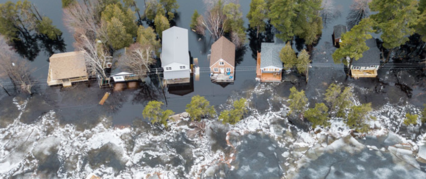
Australian banks are exposed to potential credit losses from the physical risks of extreme climate events such as fires, floods, droughts and cyclones (acute physical risks). They are also exposed to the more persistent but gradually emerging effects from rising temperature, rainfall and sea level (chronic physical risks). One potentially large exposure from climate change is mortgages, which account for approximately two-thirds of Australian major banks' portfolios. Banks lend using the current value of housing as collateral. If current values do not fully reflect the longer-term risks of climate change, housing prices could decline, leaving banks with less protection than expected against borrower default. A number of international studies have indicated that there is little evidence of climate change being fully priced into ‘at risk’ properties, even in highly vulnerable areas like the US state of Florida (Keys and Mulder 2020; Bernstein, Gustafson and Lewis 2019). As a result, the price of properties considered to be at ‘high risk’ of being affected by climate events could decline sharply and banks could experience significant credit losses if borrowers default. This is particularly the case if properties are uninsured or underinsured.[1]
To estimate the extent to which Australian banks may have mortgage exposure to climate physical risks, we combine disaggregated climate risk forecasts with micro-level data on banks' mortgage exposures. The physical risk analysis discussed below is based on data by XDI-Climate Valuation – a widely used consultancy that generously supplied these data on request. These forecasts use the Network for Greening the Financial System (NGFS) Representative Concentration Pathway (RCP) 8.5 ‘Hot House World’ scenario.[2] This is one of the scenarios recommended by the Task Force on Climate-related Financial Disclosures (TCFD 2020) for conducting scenario analysis on the impacts of climate-related risks, as well as by other international regulatory agencies. It is also one of the scenarios used in the CVA to examine banks' exposures to physical risks. The XDI-Climate Valuation data assess the climate risks to five hazards in Australia: riverine flooding, coastal inundation, forest wildfires, wind storms (other than cyclones), and ground subsidence in drought. These forecasts are generated at the address level, but the analysis that follows uses forecasts aggregated by suburb. These climate data were combined with banks' mortgage exposures from the Reserve Bank of Australia's loan-level securitisation database.
Material declines in housing prices are likely to be concentrated in specific regions
The main risk indicator used in this analysis is properties' Value at Risk (VaR). The VaR is measured by the technical insurance premium, which captures the annual expected cost of climate-related damage relative to the replacement cost of dwellings.[3] Hence, the VaR captures the costs associated with servicing housing, including insurance, repairs, replacement and maintenance costs. It does not reflect a decline in the value of the property itself. For example, a VaR of 0.5 per cent is equivalent to an annual premium of $2,500 on a building that would cost $500,000 to replace. XDI-Climate Valuation forecasts a VaR for each dwelling in Australia, which they then aggregate by suburb, providing a standardised metric for consistency and comparison. From this, we can derive which regions are forecast to experience large increases in the level of climate risk over time and the resulting impact on property valuations. Consistent with international experience, a dwelling is classed as being a ‘high risk’ property if its VaR exceeds 1 per cent (based on the US Federal Emergency Management Agency's thresholds for government insurance schemes).
Around 3½ per cent of dwellings in Australia currently have a VaR greater than 1 per cent, according to XDI-Climate Valuation; this is projected to increase to 8 per cent over the next 80 years. However, when thinking about the risk to banks' collateral exposures in climate-sensitive regions, it is the rise in climate risk yet to be reflected in property prices that is relevant. One way of quantifying this is to calculate the increase in natural disaster costs from climate risk – measured by the change in VaR from 2021 – and then translate this to decreases in housing prices over time. This identifies properties that are not considered to be ‘at risk’ currently, but are predicted to become an emerging risk in the future. Using a user cost framework, we estimate that a VaR change of 0.4 percentage points is equivalent to roughly a 10 per cent decline in housing prices due to climate risk.[4] These increases in premium costs would be incurred every year, and therefore could result in sizeable declines in property values.
Graph 1 shows the distribution of projected VaR changes across all suburbs from this approach, ranked from lowest to highest. Based on the RCP 8.5 scenario and this specific method, the majority of properties are expected to experience very little impact from climate change. By 2050, only around 1½ per cent of properties are projected to experience a rise in annual insurance premiums that could reduce housing values by around 10 per cent or more (see orange dashed line in Graph 1).[5] This increases to 9 per cent of properties by 2100 (of which 3 per cent are projected to experience up to a 20 per cent reduction in housing prices; i.e., VaR change of 1 percentage point or more, see green dashed line in Graph 1). However, there are some properties that could see very large price falls. These risks could emerge more rapidly if buyers start to recognise the increasing risk of climate change and factor this in to current property prices (by discounting prices more heavily than the actuarial fair amount) ahead of climate change impacts being fully realised.

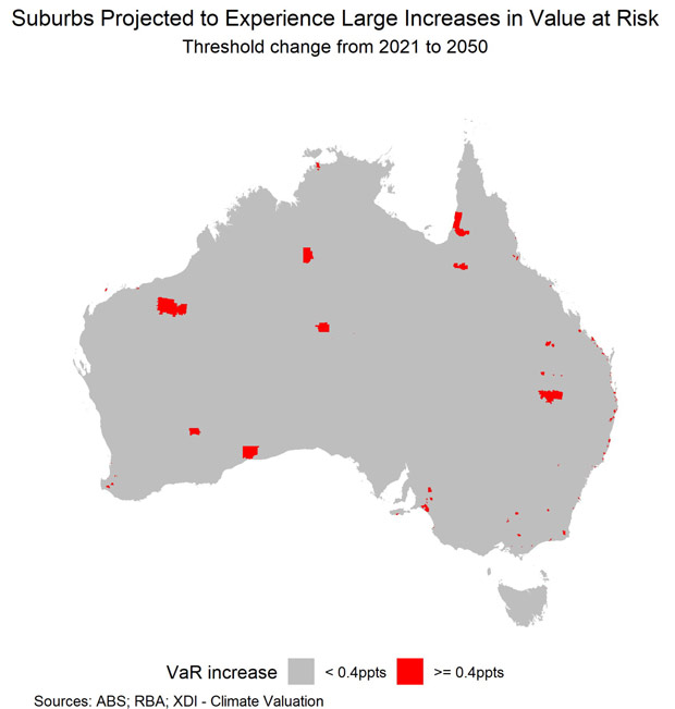
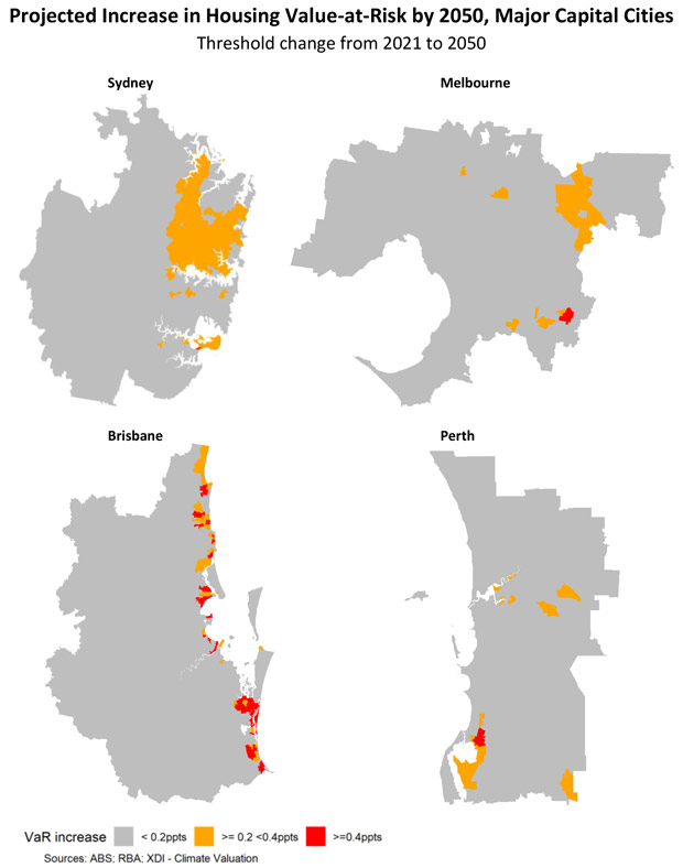
The risks also appear to be concentrated in small geographical areas, mostly in agricultural or coastal regions. This analysis suggests there are 254 climate-sensitive suburbs in 2050 with a VaR increase greater than 0.4 percentage points (and 1,438 suburbs by 2100) (Graph 2). Within the major capital cities, where the majority of properties are located, the highest risk regions are mostly located on the coastline, particularly in Brisbane (Graph 3). The risks in these regions could further increase if the affected communities find that access to, or affordability of, insurance becomes a challenge. That is, the technical insurance premium may understate the actual rise in premiums, particularly if insurers become more concerned about exposures to ‘high risk’ regions. This may arise because many of the addresses within these regions are impacted by the same hazard (e.g. an entire town is built in a flood zone or near fire hazards). In addition, if climate change causes incomes in these regions to also decline, it would result in even larger risks to banks.
The number of ‘high risk properties’ could grow
The above analysis could understate banks' actual exposure to the risks of climate change by aggregating high and low risk properties within a suburb. As a cross check, we looked at more granular property-level data provided by XDI-Climate Valuation. This alternative metric estimates the share of ‘high risk’ properties (HRP) (where the VaR is greater than 1 per cent) within each postcode. In principle, any HRP should be able to be insured, but if a large number of insurers increase annual premiums or withdraw their coverage of certain climate-sensitive regions, this may leave households without insurance cover and banks susceptible to borrower defaults. Evidence of this has already started to emerge in northern Australia, where high, unaffordable premiums are leading to a rise in uninsured homes (ACCC 2019).
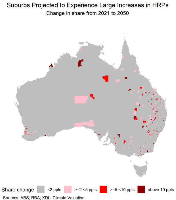
Using only HRP in our calculations produces qualitatively similar results, suggesting that there is unlikely to be much aggregation bias in our earlier estimates. Nationally, only around 0.5 per cent of properties (or 74,000 properties) are projected to move into the ‘high risk’ category by 2050. This figure is less than the share of properties for which the rise in VaR implies a 10 per cent or larger decline in house prices. Graph 4 shows suburbs where the rise in the share of HRPs is greater than or equal to 2, 5 or 10 percentage points. The regions with the largest rise in the proportion of properties that are projected to be high risk continue to include some populous regions in south-eastern Queensland and northern New South Wales, which have a large number of houses at risk of coastal inundation (Graph 4).
Falling collateral values could increase borrower leverage
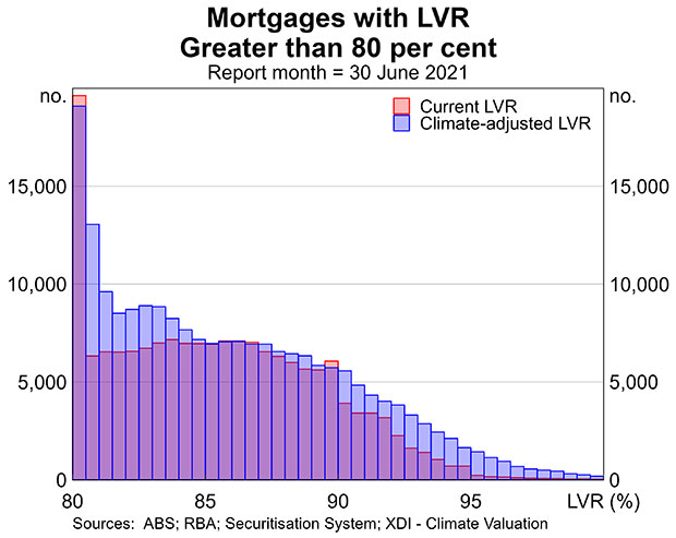
To estimate the potential impact of climate change on banks' mortgage books, we translated the potential falls in housing prices in climate-sensitive suburbs (by 2050) into an implied change in borrower leverage, as measured by loan-to-value ratios (LVR). To do this, we used the current balance of outstanding mortgages and property values in the Reserve Bank's securitisation database and adjusted for the projected housing price impact of climate change from the earlier exercise.[6] These data were matched on a more aggregated, postcode-level basis (rather than suburb level). Using this approach, our results suggest that climate change results in around 40,000 more loans (2¼ per cent of all loans) having an LVR greater than 80 per cent (Graph 5). Within this, around half of these loans move to an LVR greater than 90 per cent. The majority of these risks appear to be concentrated in banks with greater exposure to particular NSW and QLD regions, rather than the major banks (who hold fewer mortgages in these regions).
Limitations
There are a number of limitations to this method that may affect our findings. The risks to banks' portfolios may be overstated in this exercise because we assume that banks' exposures will not change in the future. In reality, banks are expected to increasingly incorporate climate risks into their lending decisions (not just whether they will lend on a particular property, but how much). The VaR measure also excludes land values and so likely overstates the impact of higher technical insurance premiums on housing prices (because the denominator is understated when it only captures the value of the building). We are also unable to combine these estimates of impacts on the collateral backing bank loans with information on how climate change might impact the probability of default on mortgages. Banks will typically sustain losses only if both collateral values and borrower income decline. On the other hand, the risks to bank portfolios may be understated by other factors. For example, we implicitly assume rents are unaffected by climate change, but there may be less demand to rent houses that are at risk of damage. The need to aggregate some of our data may also result in some understatement of risks. More broadly, there is considerable uncertainty around predicting the future impacts of climate change, as a number of variables could cause the actual result to differ materially. This means caution should be taken when interpreting these results.
The transition risks for bank business lending
Australian banks also face credit risk through their lending to businesses that are exposed to transition risk. This risk is likely to be broadly proportionate to the emissions intensity of each industry they lend to – whether those emissions are from the industry itself or indirectly through the industry's supply chain. For example, firms that directly emit large quantities of greenhouse gases (relative to their income) are clearly exposed to transition risk.[7] But so too are firms that are heavy users of the output of emissions-intensive industries because they could experience higher prices if the cost of carbon abatement is passed on. Food manufacturers are an example of this as their direct emissions are relatively small but they use products from the emissions-intensive agriculture industry.
Our analysis incorporates both the direct and indirect channels to provide a more accurate estimate of Australian banks' exposure to the transition risks of climate change. It is assumed the risk is proportionate to emissions intensity. We combined estimates of emissions by 114 sub-industries (using the Australian Bureau of Statistics input-output table industry groups) with disaggregated data on bank exposures by (SIC-3) industry, sourced via a special request from the major banks. Data on emissions by industry were primarily sourced from Australia's National Greenhouse Gas Inventory database, the National Greenhouse and Energy Reporting scheme and with some additional assumptions. By combining these data with disaggregated data on bank exposures by sub-industry, we calculated three measures of emissions intensity to investigate the extent of industry transition risks:
- Scope 1 emissions: data for each sub-industry were used to calculate direct emissions intensity, defined as emissions per dollar of Australian production.
- Scope 2 emissions: we added the input-weighted sum of emissions of industries that directly supply each industry to the direct emissions of that industry. For example, when calculating retail trade emissions, it also captures the emissions of the wholesale industries that directly supply the retail industry.
- Scope 3 upstream emissions: this measure captures the emissions from the complete supply chain of each industry. For example, when calculating retail trade emissions it also captures the emissions of the transport industry that supplies goods to the wholesale industry that are then distributed via the retail industry.
We recognise that this method is just one way of estimating the size of exposures to emission-intensive industries. Notably, the scope 3 (upstream) measure does not consider the downstream emissions from customers. For example, the combustion of coal in coal-fired electricity generators is not captured as a relevant downstream scope 3 emissions source for coal mines and coal logistics (although it is captured at an economy level through electricity emissions), nor are the emissions from Australian coal used in overseas generation.[8]
Electricity, agriculture and manufacturing appear to be the most emission-intense industries …
Graph 6 shows the emissions intensity of the most emissions-intensive industries. According to this approach, the most emissions-intensive industries (by scope 1 emissions) are electricity and parts of agriculture (specifically sheep, grains and cattle), with a wide range of manufacturing industries and oil & gas extraction comprising the remainder of the top 20 industries.[9] These specific industries could all face considerable disruptions as Australia (and the world) transitions to a lower-emissions economy, with subsequent flow-on effects to banks' business books. Another set of industries could also be affected because of their indirect emissions through their supply chain. Several industries that are not incorporated in the top 20 by direct emissions are captured in the top 20 by scope 3 emissions. The meat and dairy manufacturing industries and iron & steel manufacturing see a very large increase in their emissions intensity when the emissions embodied in their supply chains are taken into account. For the meat and dairy industries, the scope 2 and scope 3 emissions reflect the reliance of these industries on the sheep, grain and cattle industry, while the iron & steel industry's reliance on coal contributes to its scope 3 emissions. These industries could therefore have a higher exposure to transition risk due to the industry composition of their supply chains.

… but banks' exposures to these emissions-intensive industries seem relatively small
As Australian industries look to transition towards cleaner production methods, the level of disruptions to the banking system will directly depend on the size of exposures banks have to these emissions-intensive industries. If this proves to be material, it could have systemic consequences for the resilience of banks. To investigate this, we combine these emissions data with data on the scale of banks' business lending exposures.
The disaggregated industry exposure data we obtained from the major banks show that the majority of their lending exposures are to industries that look to be less emissions intensive. Specifically, Graph 7 indicates that banks' lending to industries with a high level of emissions (i.e. those to the right of the graph) are typically small, while their largest exposures (i.e. those to the top of the graph) are to industries with relatively low emissions intensity. (We exclude lending to finance from this graph because the risks associated with these exposures are of a different nature.) The largest risks to banks appear to come from industries like electricity, agriculture and oil & gas, reflecting that these industries have both relatively high emissions and that banks have reasonably sizeable exposures to them.[10]

From this analysis, around 20 per cent of banks' business loans are found to be to industries with (scope 1) carbon emissions per dollar of output that are in in the top quartile of all industries by emissions (Graph 8). Based on this approach, banks' current portfolio of loans is estimated to be somewhat less emissions intensive than the economy as a whole. In saying that, the income of some borrowers in these industries is likely to decline quickly if government policies (domestic or international) around greenhouse gas emissions or consumer preferences for ‘green’ products shift rapidly. Should income decline more quickly than the borrower expected over the life of the loan, this could result in a sizeable impact on banks' business lending books. Nevertheless, the majority of banks' business lending is extended with a term of less than five years, in part due to the large capital costs associated with long-term lending (maturity is a component of business risk weight calculations).

Understanding how much risk these exposures pose to banks is complicated, and depends on:
- the ability of exposed firms to absorb potential future emissions pricing in their profit margins or to pass it onto consumers
- their opportunities and costs to reduce emissions
- whether they might receive any compensation during the transition.
Each of the major banks also have climate change policies that will further control their exposure to emissions-intensive industries over coming years (such as the thermal coal, oil & gas industries).
Limitations
Our estimates of the risk facing banks are affected by the aggregation at the sub-industry level and the range of assumptions used. Most importantly, modelling emissions intensity at the industry level implicitly assumes that all firms within an industry have the same emissions intensity. This limitation is greatest when there are multiple methods of producing the same output within an industry, some of which are more emissions intensive than others. A prominent example of this is that lending to renewables electricity generation is assumed to have the same emissions intensity (and hence risk) as lending to fossil fuel generators in this analysis because they are both categorised as part of the electricity generation industry. Another example is lending to the sheep, grain and cattle industry, since sheep and cattle raising are emissions-intensive activities while grain is not (but often occurs on the same farm). It is also possible that banks' credit assessment processes result in banks' exposures being focused on firms with more climate-friendly production processes than the industry average. Finally, our scope 3 emissions estimates only include upstream emissions, and not downstream emissions. By definition, these estimates will then exclude the risks to firms that sell to ‘at risk’ industries.
Discussion
The focus of banks on climate risks faced by their customers has increased significantly in recent years. This reflects banks', and regulators', increased recognition of significant physical and transition risks from climate change, which, if left unmanaged, could become substantial. The methods and datasets used in this work suggest that the risks facing domestic banks appear manageable, but there are considerable uncertainties and limitations to this analysis. Projected costs from weather-related loan losses to banks over the next few decades could be mitigated if the majority of mortgaged properties are not in regions with elevated physical risks associated with climate change (such as coastal erosion or flooding). Similarly, this preliminary work suggests that Australian banks may have less exposure to emissions-intensive industries relative to the economy as a whole. The considerable uncertainty about the exact magnitude of the impacts from climate change makes it essential that banks further integrate climate risk into their mortgage and business lending processes and report on it to enable external assessment of the risks. In recognition of this, APRA has developed a Prudential Practice Guide (‘CGP 229 Climate Change Financial Risks’) designed to assist banks, insurers and superannuation trustees on managing the financial risks of climate change (APRA 2021).
Even abstracting from the uncertainties of projecting future weather events, there are also clear limitations to this work. We used simplified methods to gain some insight into the scale of banks' exposures to future physical and transition risks. We were also unable to consider the impact of climate change on household income. Finally, this work is based off a snapshot of banks' current housing and business lending portfolios, which will almost certainly be materially different in the future, particularly as more management actions are put in place. Accordingly, this work is just one way of examining the climate exposures facing Australian banks, and should be viewed as an initial assessment that will be improved upon by the more detailed and in-depth analysis of the upcoming CVA. Nevertheless, having multiple approaches to investigating the potential impacts of climate change is important in an environment of growing uncertainty and constant change.
Footnotes
The authors undertook this work while in the Financial Stability Department. They would like to thank Natasha Cassidy, Guy Debelle, Michelle Lewis, Jonathan Kearns, Marcus Miller, Anna Park, Penny Smith and Callan Windsor for their valuable assistance and contributions. They would also like to thank XDI-Climate Valuation and the four major banks who supplied data for this work. [*]
See FSB 2020. [1]
RCP 8.5 is the concentration of greenhouse gas emissions that increases planetary warming by an average of 8.5 watts per square metre across the planet, resulting in a temperature increase of about 4.3˚C by 2100. [2]
The technical insurance premium (TIP) is defined here as the annual average loss per address (or group of addresses) for all hazard impacts; the actuarially fair premium – meaning the premium is equal to expected claims, not the actual premium. The TIP is based on the cost of damage to an asset, expressed in 2020 dollars with no discounting or adjustments for other transaction costs. [3]
The user cost framework proposes that the ‘user cost’ of owning a home should be equal to the rental yield if prices are at their ‘fundamental’ value (Fox and Tulip 2014). An increase in climate change risk and the associated increase in insurance premium should increase the rental yield and lead to a reduction in housing prices. In this scenario, we assume a starting rental yield of 4 per cent and the VAR increases by 0.4 percentage points. This increases the user cost or rental yield and leads to a fall of 10 per cent in house prices. [4]
This mapping from the technical insurance premium to housing prices is based on the user cost framework, which assumes that the rental yield on housing is equivalent to the cost of owning a house (interest, depreciation, insurance, etc), adjusted for capital gains. The mapping shown here assumes all costs other than insurance remain stable (including rents, which would arguably fall for climate-affected properties), and holds current rental yields constant into the future. [5]
‘Current balance’ includes the outstanding amount of the loan, as at the collateral date. It is the sum of the outstanding amount on the loan, unpaid and due principal, interest, any penalty interest, and all other fees and costs charged to the loan balance. [6]
Greenhouse gases (such as carbon dioxide) contribute to the greenhouse effect by absorbing infrared radiation. [7]
Kemp, McCowage and Wang (2021) discuss the implications for Australia's fossil fuel exports from net zero emissions policies in the Asian region. [8]
The coal industry does not appear on this list because it does not emit much carbon when it is mined. However, coal releases significant emissions when it is burned (for electricity, domestically or overseas). Fugitive emissions have been excluded from this assessment. [9]
According to the publicly available figures for FY2020, the major banks' total coal mining exposures is approximately $2.3 billion; oil & gas extraction exposures are around $25 billion. [10]
References
ACCC (Australian Competition and Consumer Commission) (2019), ‘High Premiums Leading to a Rise in Uninsured Homes in Northern Australia’, Media Release No 251/19, 20 November. Available at <https://www.accc.gov.au/media-release/high-premiums-leading-to-rise-in-uninsured-homes-in-northern-australia>.
APRA (Australian Prudential Regulation Authority) (2021), ‘CGP 229 Climate Change Financial Risks’, Prudential Practice Guide, April. Available at <https://www.apra.gov.au/sites/default/files/2021-04/Draft%20CPG%20229%20Climate%20Change%20Financial%20Risks_1.pdf>.
Bernstein A, M Gustafson and R Lewis (2019), ‘Disaster on the Horizon: The Price Effect of Sea Level Rise’, Journal of Financial Economics, 134(2), pp 253–272. Available at <https://www.sciencedirect.com/science/article/pii/S0304405X19300807>.
Climate Valuation (Cross Dependency Initiative) (2019), ‘Climate Change Risk to Australia's Built Environment: A Second Pass National Assessment’, October. Available at <https://xdi.systems/wp-content/uploads/2019/10/Climate-Change-Risk-to-Australia%E2%80%99s-Built-Environment-V4-final-reduced-2.pdf>.
FSB (Financial Stability Board) (2020), ‘The Implications of Climate Change for Financial Stability’, 23 November. Available at <https://www.fsb.org/wp-content/uploads/P231120.pdf>.
Fox R and P Tulip (2014), ‘Is Housing Overvalued?’, RBA Research Discussion Paper No 2014-06.
Kemp J, M McCowage and F Wang (2021), ‘Towards Net Zero: Implications for Australia of Energy Policies in East Asia’, RBA Bulletin, September.
Keys B and P Mulder (2020), ‘Neglected No More: Housing Markets, Mortgage Lending, and Sea Level Rise’, NBER Working Paper No 27930, October. Available at <https://www.nber.org/system/files/working_papers/w27930/w27930.pdf>.
RBA (2021), ‘Box B: Supply Chains During the COVID-19 Pandemic’, Statement of Monetary Policy, May.
TCFD (Task Force on Climate-related Financial Disclosures) (2020), ‘2020 Status Report’, October. Available at <https://www.fsb.org/wp-content/uploads/P291020-1.pdf>.