RDP 2014-12: A State-space Approach to Australian GDP Measurement 4. Results
October 2014 – ISSN 1320-7229 (Print), ISSN 1448-5109 (Online)
- Download the Paper 904KB
4.1 Model 1: No Correlation
In Model 1 we assume that shocks to GDP and the measurement errors are independent of each other. Table 1 shows the parameter estimates.
| Parameter | Distribution | Prior | Posterior | |||||
|---|---|---|---|---|---|---|---|---|
| Mean | Std dev | Mode | Median | 5% | 95% | |||
| GDP equation | ||||||||
| μ | Normal | 0.80 | 10 | 0.79 | 0.78 | 0.62 | 0.95 | |
| ρ | Beta | 0.50 | 0.2 | 0.37 | 0.40 | 0.24 | 0.56 | |
| Exogenous processes | ||||||||
 |
Inv Gamma | 2 | 4 | 0.38 | 0.39 | 0.29 | 0.52 | |
 |
Inv Gamma | 2 | 4 | 0.43 | 0.44 | 0.34 | 0.57 | |
 |
Inv Gamma | 2 | 4 | 0.68 | 0.71 | 0.56 | 0.89 | |
 |
Inv Gamma | 2 | 4 | 0.29 | 0.31 | 0.24 | 0.42 | |
| Marginal data density −516.61 | ||||||||
The median estimate of μ is 0.78, which is close to the average growth rate of GDP(A) over the sample. The estimate of ρ is 0.40. This implies that the GDP growth process has relatively little persistence, although the parameter is larger than estimates from an AR(1) model of GDP(A) growth over our sample. Innovations to GDP growth are estimated to be similar in size to the measurement errors in the expenditure and production equations, and smaller than the average measurement errors in the income equation.
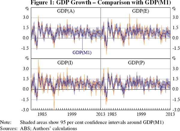
Using the posterior distribution of the model's parameter values, we can recover an estimate of ‘true’ GDP growth over the sample. We call this series derived from Model 1 GDP(M1). Figure 1 compares this estimate to the published quarterly growth rates of GDP(A), GDP(E), GDP(I) and GDP(P). GDP(M1) is highly correlated with GDP(A), but it is less volatile.[12] That is, our model suggests that some extreme readings of GDP(A) are likely to represent measurement error in one or more of the individual measures of GDP. Our methodology also allows us to construct confidence bands around the GDP growth estimates, which are also shown in Figure 1. These are generally wide. For example, in the June quarter of 2013, our model's median estimate of GDP growth was 0.6 per cent, and the 95 per cent confidence bands spanned 0.1–1.2 per cent.
4.2 Model 2: Correlation
In Model 2, we allow for correlation between innovations to GDP and the measurement errors. Table 2 presents the parameter estimates.
| Parameter | Distribution | Prior | Posterior | |||||
|---|---|---|---|---|---|---|---|---|
| Mean | Std dev | Mode | Median | 5% | 95% | |||
| GDP equation | ||||||||
| μ | Normal | 0.80 | 10 | 0.79 | 0.79 | 0.63 | 0.94 | |
| ρ | Beta | 0.50 | 0.2 | 0.47 | 0.46 | 0.26 | 0.67 | |
| Exogenous processes | ||||||||
 |
Inv Gamma | 2 | 4 | 0.39 | 0.43 | 0.31 | 0.56 | |
| σGE | Normal | 0 | 10 | −0.25 | −0.27 | −0.48 | −0.09 | |
| σGI | Normal | 0 | 10 | −0.17 | −0.18 | −0.46 | 0.10 | |
| σGP | Normal | 0 | 10 | −0.13 | −0.16 | −0.35 | −0.02 | |
 |
Inv Gamma | 2 | 4 | 0.84 | 0.91 | 0.56 | 1.35 | |
| σEI | Normal | 0 | 10 | 0.37 | 0.39 | 0.10 | 0.74 | |
| σEP | Normal | 0 | 10 | 0.31 | 0.36 | 0.11 | 0.66 | |
 |
Inv Gamma | 2 | 4 | 0.92 | 0.98 | 0.58 | 1.46 | |
| σIP | Normal | 0 | 10 | 0.17 | 0.20 | −0.07 | 0.52 | |
 |
Inv Gamma | 2 | 4 | 0.45 | 0.52 | 0.29 | 0.88 | |
| Marginal data density −514.53 | ||||||||
The estimated parameters of the GDP process, µ and ρ, are similar to those in Model 1. However,
the variance of innovations to GDP and the measurement errors are larger. This
is most notable in the expenditure equation, where the variance of the measurement
errors is now similar in magnitude to the income equation. This is not an artefact
of the restriction imposed in Equation (3); varying the restriction, or applying
it to GDP(P) rather than GDP(E), leaves the value of  largely unchanged.
In contrast, the variance of the measurement errors in the production equation
remains around the same size as for the estimated GDP innovations.
The covariances between the measurement errors are positive, and generally statistically significant. This is consistent with the fact that information from some surveys feed into more than one measure of GDP. In contrast, covariances between innovations to GDP and the measurement errors are generally negative and statistically significant. This suggests that the characteristics of measurement errors vary over the business cycle, perhaps because the types of challenges the ABS faces in measuring GDP growth vary across the business cycle. In general, the fact that the covariances of innovations to GDP and measurement errors are statistically significant highlights the importance of controlling for these correlations when evaluating the pace of economic growth.
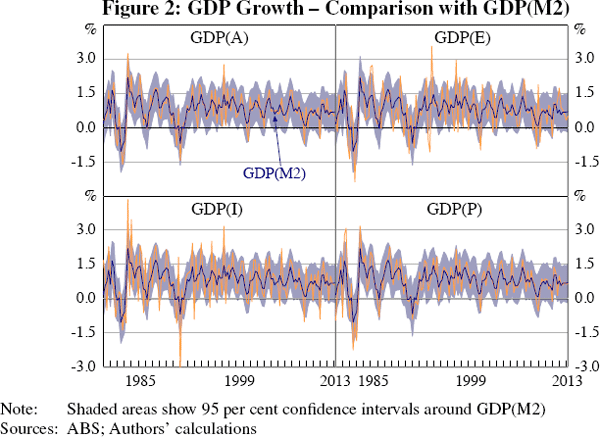
Figure 2 shows the plot of GDP derived from Model 2, GDP(M2). This measure is considerably smoother than GDP(A). This reflects the fact that when we allow for correlation between shocks some large changes in multiple measures are attributed to measurement error rather than treated as signal.
4.3 Model 3: Unemployment
In Model 3 we include the quarterly change in the unemployment rate as an additional observable variable. Table 3 presents the parameter estimates.
| Parameter | Distribution | Prior | Posterior | |||||
|---|---|---|---|---|---|---|---|---|
| Mean | Std dev | Mode | Median | 5% | 95% | |||
| GDP equation | ||||||||
| μ | Normal | 0.80 | 10 | 0.79 | 0.79 | 0.59 | 1.01 | |
| ρ | Beta | 0.50 | 0.2 | 0.65 | 0.62 | 0.46 | 0.77 | |
| Unemployment equation | ||||||||
| κ | Normal | 0 | 10 | 0.54 | 0.51 | 0.38 | 0.82 | |
| λ | Normal | −0.50 | 10 | −0.69 | −0.64 | −1.03 | −0.50 | |
| Exogenous processes | ||||||||
 |
Inv Gamma | 2 | 4 | 0.24 | 0.28 | 0.19 | 0.46 | |
| σGE | Normal | 0 | 10 | 0.00 | −0.01 | −0.11 | 0.05 | |
| σGI | Normal | 0 | 10 | −0.03 | −0.04 | −0.14 | 0.03 | |
| σGP | Normal | 0 | 10 | −0.04 | −0.05 | −0.14 | 0.01 | |
| σGU | Normal | 0 | 10 | 0.12 | 0.12 | 0.07 | 0.21 | |
 |
Inv Gamma | 2 | 4 | 0.63 | 0.70 | 0.54 | 0.88 | |
| σEI | Normal | 0 | 10 | 0.25 | 0.23 | 0.10 | 0.40 | |
| σEP | Normal | 0 | 10 | 0.19 | 0.22 | 0.11 | 0.34 | |
 |
Inv Gamma | 2 | 4 | 0.80 | 0.87 | 0.69 | 1.10 | |
| σIP | Normal | 0 | 10 | 0.09 | 0.11 | 0.00 | 0.24 | |
 |
Inv Gamma | 2 | 4 | 0.42 | 0.47 | 0.36 | 0.60 | |
 |
Inv Gamma | 0.3 | 4 | 0.08 | 0.08 | 0.05 | 0.21 | |
| Marginal data density −510.43 | ||||||||
The estimated mean parameter for the GDP process is similar to the previous models, although GDP growth has more persistence than in Models 1 and 2. The coefficients in the unemployment equation suggest that a 1 percentage point increase in the rate of quarterly GDP growth lowers the unemployment rate by around 0.6 percentage points, which is slightly above existing Okun's law estimates for Australia (Borland 2011).
The parameter estimates for the shock processes differ from the previous models' in two respects. First, the variance of GDP innovations is much smaller when we include the unemployment rate as an observable variable in the model. Second, the negative correlation between GDP innovations and measurement errors in the GDP(M2) measurement equations largely disappears. However, the covariances between the measurement errors remain positive and statistically significant.
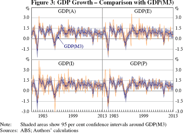
Figure 3 compares this model's estimate of GDP growth, GDP(M3), to the published figures. Overall, the results for Model 3 are similar to those of Model 2 as, once again, our measure of GDP is smoother than GDP(A). The greatest difference lies in the recessions of the early 1980s and 1990s and the slowdown associated with the global financial crisis in the late 2000s. The inclusion of the unemployment rate, which increased in all three episodes, lowers Model 3's estimate of GDP growth relative to the estimates in Models 1 and 2 that do not include the unemployment rate.
4.4 How Do Our Measures Compare with the Published Trend Measure of GDP?
Our methodology provides measures of GDP growth that incorporate information about the degree of noise generated by measurement error in the published estimates. The result is a smoother measure. The ABS also produces a smoother measure of output growth, constructed by applying a Henderson moving average to GDP(A). The ABS publish the resulting measure, known as ‘trend’ GDP, at a quarterly frequency. Figure 4 compares the ABS trend GDP with the measures introduced in this paper.
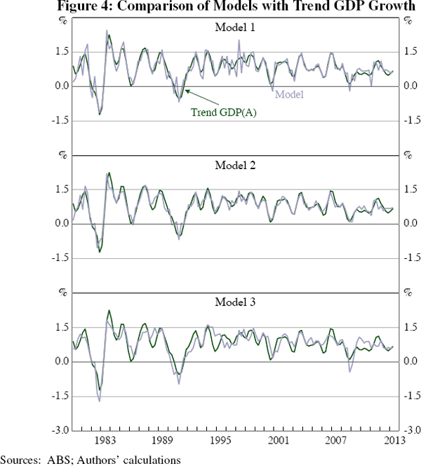
The histories of the series are generally quite similar, which is encouraging. Trend GDP(A) has a disadvantage relative to our method, however, in that it suffers from end-point problems. The Henderson trends used by the ABS apply moving averages to past and future observations in a series. As the series approaches its end point, there are fewer observations upon which to calculate these averages. While the ABS takes steps to ameliorate this issue, recent trend GDP data remain subject to substantial revision as new data are received.[13] In Section 5, we demonstrate that the techniques presented in this paper appear to be less affected by end point problems and so should provide users with a better indication of output growth in real time.
4.5 What are the Relative Contributions of GDP(E), GDP(I) and GDP(P)?
At its core, our methodology represents an alternative way of combining the information in the three existing ABS measures of GDP growth. One might wonder how our models weight each of the three measures and the extent to which this differs from the simple average used to construct GDP(A). We answer these questions in two ways: first we examine Kalman gains; and second we find the weighted average of GDP(E), GDP(I) and GDP(P) that is closest to our measure of GDP growth.
4.5.1 Kalman gains
Kalman gains govern the extent to which our models adjust their estimates of the rate of GDP growth in light of new observations of GDP(E), GDP(I) or GDP(P). If the Kalman gain on a particular measure of GDP is large then the model extracts a large amount of signal from new data on that measure. For example, the model will interpret a large increase in the growth rate of an observed GDP measure that has a large Kalman gain as a signal that GDP growth has increased. In contrast, it will consider a similar increase in the growth rate of an observed GDP measure that has a small Kalman gain as being more likely to reflect measurement error.
For each draw from the posterior distribution of model parameters, we can recover an estimate of the Kalman gain for each observable variable. Figure 5 summarises these Kalman gains for Model 3.[14] In the figure, each blue dot compares the Kalman gains of two measures of GDP for an individual draw from the posterior distribution. The red dot and circle represent the posterior median and 90 per cent probability interval for each pair. Intuitively, if most dots lie to the left of the dashed 45 degree line, then the Kalman gain for the observed GDP measure on the vertical axis is greater than that of the measure on the horizontal axis, and vice versa. A mass of dots surrounding the dashed 45 degree line indicates that the model puts roughly equal weight on the two observed measures of GDP.
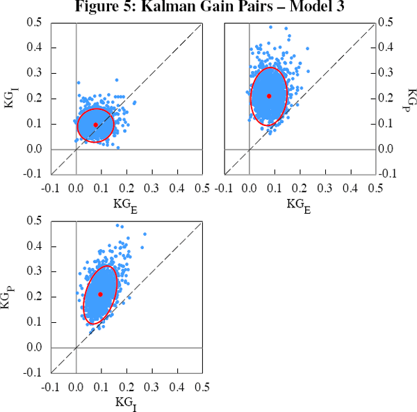
Figure 5 confirms that the model places more weight on GDP(P) than on the other two measures. It also places roughly equal weight on GDP(E) and GDP(I). This is consistent with the fact that the estimated measurement errors in the production equation are considerably smaller than those in the expenditure and income equations.
4.5.2 Closest convex combination
The second way in which we gauge the relative importance of the three observed measures of GDP is by calculating the fixed-weight combinations of the three measures that come closest to replicating our measures of GDP growth. That is, we calculate the values of α1 and α2 that solve:[15]
Table 4 shows the weights for each model.
| Weight on | Model 1 | Model 2 | Model 3 |
|---|---|---|---|
| GDP(E) | 0.30 | 0.09 | 0.22 |
| GDP(I) | 0.21 | 0.26 | 0.24 |
| GDP(P) | 0.49 | 0.65 | 0.54 |
Consistent with the results in the Kalman gain section, it appears that our models extract more information from GDP(P) than from the other two measures of GDP. However, there is some discrepancy in the relative weight attached to the other two measures. Model 1 places relatively more weight on GDP(E) than GDP(I), while Model 2 does the reverse and Model 3 places roughly equal weight on the two measures.
4.6 GDP Behaviour during Slowdowns
Although our measures of GDP exhibit similar cycles to GDP(A), the quarterly growth rates differ. These differences are most relevant around business cycle turning points, when distinguishing signal from noise in GDP growth is of greatest importance. In this section, we discuss the behaviour of our models during the Australian economy's two most recent slowdowns, which occurred in 2000–2001 and 2008–2009.
In both of these episodes, GDP(A) indicates that the Australian economy experienced a large contraction in economic activity, followed by a strong recovery in the subsequent quarter. In the earlier episode, the economy returned rapidly to trend growth. In contrast, in the third quarter of the 2008–2009 episode, GDP growth slowed again, with GDP(A) expanding by a mere 0.1 per cent in the June quarter of 2009.
In the presence of measurement error, large changes in economic activity make policymaking difficult. Did the strong GDP growth recorded in the March quarters of 2001 and 2009 accurately signal that the economy had recovered from the declines of previous quarters? Or was it merely statistical noise that concealed ongoing economic weakness?
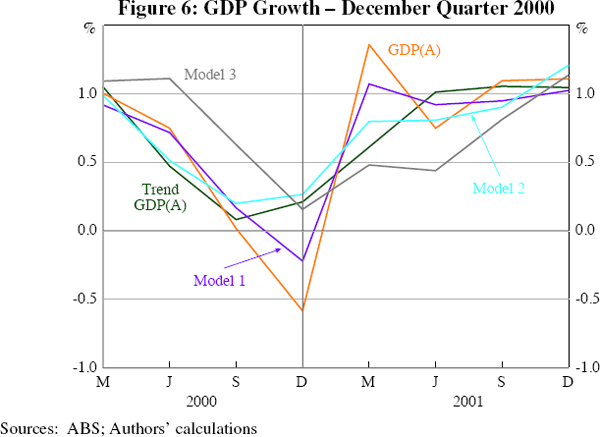
Our models suggest that neither the slowdown of 2000–2001 nor the subsequent recovery was as dramatic as the GDP(A) outcome suggests (Figure 6). Models 2 and 3 suggest that the economy experienced a period of two to three quarters of substantially below-average growth, but did not actually contract. Model 1 displays a similar quarterly pattern to GDP(A), but with less extreme movements. All of the models suggest that by early 2001 growth in economic activity had begun to recover.
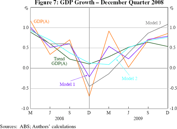
In contrast, according to our models, the slowdown of 2008–2009 was more prolonged than indicated by GDP(A) (Figure 7). Model 2 suggests that the economy experienced at least three quarters of growth substantially below average. And Model 3 records two consecutive quarters of negative growth in the December quarter of 2008 and March quarter of 2009. This is consistent with the beliefs of policymakers at the time that the Australian economy was in recession in early 2009 (Stevens 2009). All three measures assign a large proportion of the recovery in GDP(A) growth in the March quarter of 2009 to measurement error. This is consistent with the fact that the increase in GDP growth in that quarter was primarily observable in GDP(E) and GDP(I), to which the models apply relatively less weight.
4.7 Is Australian GDP Measurement Different?
A natural benchmark against which to compare our results is Aruoba, Diebold, Nalewaik, Schorfheide and Song (2013), who conduct a similar exercise using US data. Our results differ from theirs in two important respects.
First, across a number of specifications, Aruoba et al find that the average size of measurement errors in US GDP(I) is smaller than in US GDP(E). Consequently, their model places more weight on income than expenditure in constructing a measure of US GDP growth. In contrast, we find that in the Australian data measurement errors on the income side of the accounts tend to be a little larger than on the expenditure side.
A second difference is that Aruoba et al find that innovations to US GDP are on average larger than measurement errors. In contrast, we find larger relative measurement errors in Australian GDP data.
While it is hard to reach firm conclusions as to the differences between Aruoba et al (2013) and our work, we find it plausible that they could reflect differences in the structure of the US and Australian economies. Relative to the United States, Australia is a smaller and more open economy, and commodity exports are relatively more important. Given that commodity prices are typically more volatile than manufacturing or services prices, commodity exporters tend to experience greater volatility in nominal GDP – the quantity of output multiplied by its price – than other economies. This nominal volatility makes real GDP measurement on the income side of the national accounts particularly challenging, because of the need to determine appropriate deflators to apply to volatile nominal GDP flows. Similar challenges apply when measuring expenditure, in particular export and import volumes. To the extent that commodity prices and exchange rates are observable, it should be possible to deflate export and import values accurately. However, if prices and exchange rates are volatile, imposing appropriate deflators is more difficult, creating the possibility of additional measurement error. The volatility of Australian export prices could go some way to explaining the relatively large measurement errors that we report for Australian GDP(E) and GDP(I).
Footnotes
Table 5 contains descriptive statistics for all of the estimated GDP series. [12]
Of course, seasonally adjusted series may also feature end point problems if there are changes in seasonal patterns over time. [13]
The distributions for the other models are similar. [14]
Note that constructing a measure of GDP using these weights will not recover GDP(M1), GDP(M2) or GDP(M3) because the Kalman filter does more than a simple contemporaneous averaging of the GDP measures in its extraction of actual GDP growth. [15]
