RDP 2014-12: A State-space Approach to Australian GDP Measurement 2. Estimating GDP Growth

We treat GDP growth as an unobserved variable that follows a first-order autoregressive (AR(1)) process:

where Δy_t represents the growth rate of real GDP, μ is the mean growth rate of GDP, ρ indicates persistence and ε_G,t is a normally distributed innovation. It is common to model GDP growth as an AR(1) process, as growth rates are typically assumed to be homoscedastic and moderately persistent.

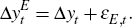
We then assume that the three observed GDP measures – GDP(E), GDP(I) and GDP(P) – provide noisy readings of actual GDP. For example, in our model the growth rate of GDP(E) is equal to the growth rate of actual GDP plus a measurement error term:

Stacking the three observed measures in matrix form gives us our measurement equation:

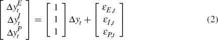
where 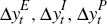represent growth in GDP(E), GDP(I) and GDP(P), and ε_E,t, ε_I,t and ε_P,t represent their measurement errors.

Using this basic framework, we estimate three models that differ in their treatment of the observable variables, the shocks to GDP and the measurement errors.

2.1 Model 1: No Correlation

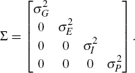
Our first model assumes that all stochastic terms are independent, that is, [ε_G,t, ε_E,t, ε_I,t, ε_P,t] ∼ N(0,Σ) where

2.2 Model 2: Correlation

Next we allow for correlation between the various GDP measures, that is, for [ε_G,t, ε_E,t, ε_I,t, ε_P,t] ∼ N(0,Σ) where

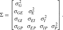
This model allows the errors in the three observable GDP measures to be interrelated, and for the size of the shock to actual GDP to affect the measurement error in the observed measures of GDP. For example, large innovations in actual GDP may be associated with less precise estimates of GDP(E), GDP(I) and/or GDP(P) than is the case for small innovations.

As shown in Appendix A, however, in order to identify the model we must place at least one restriction on the Σ matrix.^[6] In line with Aruoba et al (2013) we impose this restriction by requiring that:

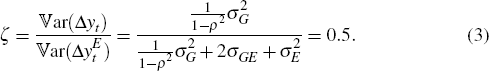
That is, we assume that the variance of actual GDP growth is equal to half of the variance of the observed GDP(E) growth series. Although intuitively appealing, the restriction is arbitrary, and any number of alternative restrictions would also suffice.^[7]

2.3 Model 3: Unemployment

Our third model includes an additional observable variable that depends on GDP growth but whose measurement error is unrelated to that of the other observable variables: the quarterly change in the unemployment rate.^[8] That is, we replace Equation (2) with

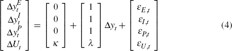
where ΔU_t is the change in the unemployment rate. In this case we assume that [ε_G,t, ε_E,t, ε_I,t, ε_P,t, ε_U,t] ∼ N(0,Σ) with

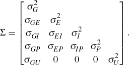
That is, we impose three restrictions on the Σ matrix – zero correlation between the measurement error of the change in the unemployment rate (ε_U,t) and the measurement error for growth of GDP(E), GDP(I) and GDP(P) (ε_E,t, ε_I,t and ε_P,t). By a similar argument to that put forward in Appendix A, the model is identified (in fact the model is over-identified).

Footnotes

The model is unidentified in the sense that with an unrestricted Σ, different model parameters can give rise to identical distributions for the observable quantities. [6]

We experimented with alternative values of ζ, and with applying the restriction to GDP(P) instead; all produced very similar results. [7]

The unemployment rate is estimated in a monthly survey of households, known as the Labour Force Survey (LFS). Measurement errors associated with these surveys are likely to be largely unrelated to errors in the quarterly GDP series, which are mainly derived from surveys of businesses and governments, although data from the LFS does feed into GDP(I). Relaxing the assumption that the correlation between measurement errors in GDP(I) and the unemployment rate is zero produces very similar results. We also estimated a model including the growth rate of employment rather than the change in the unemployment rate. Once again, this exercise produced very similar results. [8]