RBA Annual Conference – 2005 What Caused the Decline in US Business Cycle Volatility? Robert J Gordon[1]
Abstract
This paper investigates the sources of the widely noticed reduction in the volatility of American business cycles since the mid 1980s. Our analysis of reduced volatility emphasises the sharp decline in the standard deviation of changes in real GDP, of the output gap, and of the inflation rate.
The primary results of the paper are based on a small three-equation macro model that includes equations for the inflation rate, the nominal federal funds rate, and the change in the output gap. The development and analysis of the model goes beyond the previous literature in two directions. First, instead of quantifying the role of shocks in general, it decomposes the effect of shocks between a specific set of supply-shock variables in the model's inflation equation, and the error term in the output gap equation that is interpreted as representing ‘IS’ shifts or ‘demand shocks’. It concludes that the reduced variance of shocks was the dominant source of reduced business cycle volatility. Supply shocks accounted for 80 per cent of the volatility of inflation before 1984 and demand shocks the remainder. In contrast, roughly two-thirds of the high level of output volatility before 1984 is accounted for by the output errors (demand shocks) and the remainder by supply shocks. The output errors are tied to the paper's initial decomposition of the demand side of the economy, which concludes that three sectors – residential and inventory investment and federal government spending – account for 50 per cent of the reduction in the average standard deviation of real GDP when the 1950–83 and 1984–2004 intervals are compared.
The second innovation in this paper is to reinterpret the role of changes in Fed monetary policy. Previous research on Taylor rule reaction functions identifies a shift in the Volcker era toward inflation fighting with no concern about output, and then a shift in the Greenspan era to a combination of inflation fighting and strong countercyclical responses to output gaps. Our results accept this characterisation of the Volcker era but find that previous estimates of Greenspan era reaction functions are plagued by positive serial correlation. Once a correction for serial correlation is applied, the Greenspan era reaction function looks almost identical to the pre-1979 Burns reaction function!
Thus the issue in assessing monetary policy regimes comes down to Volcker versus non-Volcker. Full-model simulations show that the Volcker reaction function, if applied throughout the 1965–2004 period, would have delivered substantially higher pre-1984 output volatility than the Burns-Greenspan alternative, with the corresponding benefit of a permanent reduction in the inflation rate of 5 percentage points per annum. Compared to the succession of three reaction functions actually in effect, application of the Volcker reaction function prior to 1979 would have deepened the 1975 recession, but made the 1981–82 recession milder, since by then inflation would have been partly conquered. The paper concludes by disputing the view that better monetary policies had any role in the reduced volatility of the business cycle – the Greenspan policies did not need to fight against inflation because there was no inflation, thanks to the reversal from adverse to beneficial supply shocks, and thanks to a reduction in the size of the output errors, or ‘IS’ shifts.
1. Introduction
For well over a century business cycles have run an unceasing round. They have persisted through vast economic and social changes; they have withstood countless experiments in industry, agriculture, banking, industrial relations, and public policy; they have confounded forecasters without number, belied repeated prophecies of a ‘new era of prosperity’ and outlived repeated forebodings of ‘chronic depression’.
Arthur F Burns 1947, p 27)
The joy of macroeconomics lies not only in its intrinsic importance to the solvency of governments and the welfare of ordinary citizens, but also in its endlessly changing topics and methods. Less than 20 years ago I edited an epochal volume with a star-studded[2] cast of authors, The American business cycle (Gordon 1986), and began my introduction to that volume with support for Burns' theme that business cycles continued their ‘unceasing round’, reminding readers that the recently completed 1981–82 recession was the deepest post-war slump, and that previous conferences and comments that the ‘business cycle is obsolete’ had proved to be wildly premature.[3]
Now, the tables have turned once again. In the tradition of instant obsolescence that has always marked macroeconomic pronouncements, going back to the universal view in 1929 that an era of permanent prosperity had arrived, that 1986 volume attesting to the permanence of business cycles appeared just as the relevance of its main themes began to erode. As documented by Blanchard and Simon (2001), Stock and Watson (2002, 2004) and others, the year of our conference, 1984, marked a sharp change from high to low American business cycle volatility.[4]
The topic of this paper is the decline in the volatility of the American business cycle over the entire post-war era, defined as 1948 to early 2005. Since by almost any measure the most severe post-war business cycle was the recession of 1981–82, it is not surprising that the recent literature dates the decline in volatility at the period 1984–86, immediately after the end of that severe recession. This paper documents and reinforces the common view that the break in volatility occurred in the mid 1980s, but this paper is not about dating but rather about causes. Our examination of the decline in business cycle volatility primarily focuses on the standard deviation of changes in real GDP and on the level of the output gap, that is, the log ratio of actual to natural real GDP. We also place substantial emphasis on the even greater decline in the volatility of inflation, both because inflation is a goal of economic policy in itself, and also because volatile inflation feeds back to make output more volatile.
The set of causes that receive most emphasis in explaining the drop after 1984 in business cycle volatility is quite different from the older literature that attempts to explain why post-war (that is, post-1948) business cycles were milder than the Great Depression, or more generally, milder than all the business cycles that occurred before 1929. The earlier literature takes as its point of departure Arthur Burns' American Economics Association Presidential Address (1960). In his analysis, the first and most important cause of post-war stability was the greatly increased size of the federal government (as compared to pre-1929), particularly the automatic stabilisers inherent in government transfer payments and the personal income tax system. Also in the front rank of causes were the reduced pro-cyclical volatility of the money supply, as well as other money-related regulatory reforms, of which the 1934 introduction of federal deposit insurance must have been the most important.
But the literature on the decline in business cycle volatility within the post-war era, that is, before and after 1984, centres on quite a different set of causes. There is no discussion of the stabilising effect of the federal government, since the role of federal government spending is now recognised to be destabilising, as we will document below. Modest attention is paid to structural change, especially the shift from volatile durable goods to stable services, but there have been no suggestions that such compositional changes have contributed substantially to a reduction in overall volatility.
Rather, the ‘contest’ in the assignment of causes for the recent decline in volatility pits two worthy opponents, an improvement in the conduct of monetary policy versus a reduction in the adverse impact on macroeconomic stability of ‘shocks’. This paper provides a separate analysis of the role of demand shocks and supply shocks. The reduced volatility of demand shocks is documented by examining the volatility of the major expenditure components of GDP and their changes. We focus on the reduced volatility of federal government spending, of residential housing, and of inventory changes as important sources of improved stability, and attribute these changes respectively to the reduced share of military spending in GDP, banking and financial market reforms, and information technology that improved sales forecasts and inventory management.
This paper goes beyond the recent research, particularly Blanchard and Simon (2001) and Stock and Watson (2002, 2004), in building an explicit model that identifies and quantifies the role of supply shocks as the basic explanation of higher inflation volatility in the 1970s and 1980s, and of reduced inflation volatility in the 1990s. This inflation equation is then joined together in a simple three-equation macro model by adding a Fed reaction function and an ‘IS’ equation that quantifies the response of changes in the real GDP gap to changes in both inflation and the short-term interest rate. Using either a single equation for inflation or the three-equation model, we can quantify the effect on output and inflation volatility of both the set of supply shocks and changes in the Fed's reaction function. The role of demand shocks is quantified by examining the role of errors in the model's IS equation for the output gap.
The paper begins with quantitative evidence on several measures of business cycle volatility, turns to the role of shifts in output shares and in sectoral volatility, and then tackles the paper's major task, the estimation and simulation of the three-equation macro model with its strong emphasis on the role of supply shocks in the inflation process. The small macro model is not a symmetric VAR model. Lag lengths and the role of levels versus rates of change are handled differently in each of the equations. However, despite its simplicity, the model provides a unique quantitative assessment of the sources of reduced inflation and output volatility after 1984.
Our major conclusion is that both demand and supply shocks mattered, and changes in monetary policy mattered much less in achieving the reduced volatility of both inflation and output. A key concept in our analysis of the three-equation model is the ‘output error’ – that is, the residual variation of the output gap that cannot be explained by responses to lagged inflation and interest rates. The output error represents ‘IS shifts’ such as changes in military spending and volatile residential investment, caused by inefficient pre-1984 financial regulations and institutions. Most of the reduced volatility of inflation after 1984 was caused by the behaviour of supply shocks and the remainder by reduced volatility of the output error, that is, IS shifts. About two-thirds of the reduced volatility of the output gap is attributed to the output error, with a small remaining role for supply shocks.
Perhaps the most surprising finding in this paper is that there has been no change in monetary policy after 1990 compared to the policies pursued before 1979, taking a narrow view of policy as the response coefficients in a Taylor rule monetary policy reaction function.[5] Policy was different only in the 1979–90 Volcker interval, when fighting inflation was paramount and no weight was given to stabilising output.[6] Our results overturn other research that finds a strong emphasis on inflation fighting not just between 1979 and 1990, but after 1990 as well. We show that previous estimates of Taylor rule reaction functions are plagued by serial correlation. Once an autoregressive correction is applied to the Taylor rule equation, the post-1990 ‘Greenspan’ policy turns out to look much the same as the pre-1979 ‘Burns’ policy; both are equally different from the 1979–90 inflation-fighting ‘Volcker’ policy. If the Volcker function had been in effect throughout 1965–2004, instead of the succession of Burns-Volcker-Greenspan functions actually in effect, the fight against inflation would have started in the mid 1970s instead of 1981–82, the 1975 recession would have been deeper but the 1981–82 recession shallower, the pre-1984 volatility of the output gap about the same, and the pre-1984 rate of inflation somewhat lower.
2. Measures of Reduced Business Cycle Volatility
2.1 Four-quarter changes in real GDP
Perhaps the clearest way to become convinced of the decline in business cycle volatility over the post-war era is to study the plot in the top frame of Figure 1, showing four-quarter changes in the growth rate of real GDP over the 229 quarters between 1948:Q1 and 2005:Q1, spanning the entire quarterly database of the United States National Income and Product Accounts (NIPA). The top frame also plots a horizontal line representing the mean growth rate of real GDP over this period, which is 3.4 per cent per annum.
As shown in the top panel of Figure 1, the four-quarter percentage changes behave very differently before and after 1984. Prior to 1984, a saw-tooth pattern is evident, while after 1984 the fluctuations are much more moderate. The pre-1984 fluctuations are equally severe above and below the mean of 3.4 per cent per year. In contrast, there is nothing like this magnitude of volatility after 1984. The four-quarter growth rate of real GDP was never negative over the entire 22-year period between 1983 and 2005, except in the brief interval associated with the 1990–91 recession, namely the March to September quarters of 1991. In fact, some doubt has been cast on the NBER's declaration of a recession in early 2001, because the four-quarter change in real GDP never became negative in that episode and indeed never fell below 0.2 per cent in any quarter in 2001.
The lower panel of Figure 1 shows the rolling 20-quarter standard deviation of the four-quarter growth rate of real GDP, and highlights the decline in volatility evident in the top panel. There was a sharp and apparently permanent decline after 1987 to a range of between 0.5 and 1.5 percentage points. Because the calculation of the rolling standard deviation over a 20-quarter window causes the post-1983 drop in volatility to be reflected five years later, we can dramatise the movement toward stability by splitting the time period of the lower panel of Figure 1 at the December quarter 1987. The mean of the standard deviations plotted in the lower panel of Figure 1 is 2.8 percentage points for 1952:Q4–1987:Q4 and a much lower 1.3 percentage points for 1988:Q1–2005:Q1.
2.2 The output gap
In principle, part of the variance of real GDP changes could reflect changes in the growth rate of natural real GDP, and we would not associate these changes with business cycle volatility. The top panel of Figure 2 depicts the log output ratio, or ‘output gap’, as a percentage (100 times the log ratio of actual to natural real GDP). The dividing line of reduced output volatility at the year 1984 is not quite as stark in Figure 2 as in Figure 1, partly because the output gap is a level rather than a rate of change and thus cumulates and partially smooths out the volatile pre-1984 rates of change shown in Figure 1. However, there is still ample evidence of a decline in the volatility of the output gap after 1984. The lower panel quantifies the shift in the volatility of the output gap by plotting (in parallel with Figure 1) its rolling 20-quarter standard deviation. There is less dramatic evidence in the bottom frame of Figure 2 of a post-1984 drop in output volatility than in Figure 1. The volatility of the four-quarter changes drops by 55 per cent when 1952–87 is compared with 1988–2005, while the volatility of the output gap drops by a smaller 42 per cent.

2.3 Inflation and output volatility
An important source of high output volatility before 1984 was high inflation volatility, and we show later that the reduction of inflation volatility after 1984 made a substantial contribution to the post-1984 decline in output volatility. We will also show that high inflation volatility prior to 1984 can be linked to the behaviour of an explicit set of supply-shock variables. Figure 3 compares the 20-quarter standard deviation of four-quarter changes in real GDP and the GDP deflator, where the close relationship between output and inflation volatility is evident in the 1974–88 period. We also note that output volatility was relatively high between 1952 and 1962, despite the low volatility of inflation, and that very low inflation volatility between 2000 and 2005 did not prevent an increase in output volatility associated with the 2001 recession and subsequent recovery. (The averages of the rolling 20-quarter standard deviations for output and inflation are shown in Table 1).
| 1952:Q4–1972:Q4 | 1973:Q1–1987:Q4 | 1988:Q1–2005:Q1 | |
|---|---|---|---|
| Real GDP | 2.69 | 2.87 | 1.25 |
| GDP deflator | 1.11 | 1.67 | 0.48 |
|
Source: author's calculations |
|||
The fact that output volatility was so high between 1952 and 1972, despite relatively low inflation volatility, suggests that the role of shocks as a cause of high output volatility should include not only supply shocks but also demand shocks, including changes in military spending.
3. Sectoral Shifts in Volatility and Spending Shares
A simple method to learn about the sources of reduced output volatility is to decompose GDP into its 11 major expenditure components. We can ask which components had the greatest and least declines in volatility, and also determine if shifts in shares of spending among the components contributed to the overall reduction in volatility, for example, by a shift from volatile investment spending and federal government spending to relatively stable spending on consumer services.
The top section of Table 2 displays the standard deviation of four-quarter changes in 11 GDP expenditure components over the 1950–83 and 1983–2005 intervals.[7] In the top section of the table, only one component – non-residential structures – was more volatile in the second interval than in the first. The volatility of most components declined by less than the volatility of real GDP, indicating that the reduced volatility of total GDP was aided by an increase in the negative covariance across the components. The volatility of only two components – investment in residential structures and federal government spending – declined by more than the volatility of real GDP. Somewhat surprisingly, the volatility of inventory investment was virtually unchanged, although we subsequently qualify this conclusion with a different measurement technique.[8]
| 1950–1983 | 1984–2005 | Ratio of 1984–2005 to 1950–1983 (per cent) |
|
|---|---|---|---|
| Standard deviation of four-quarter real growth rates | |||
| Real GDP | 3.0 | 1.6 | 51 |
| Consumption of durable goods | 9.4 | 4.9 | 52 |
| Consumption of non-durable goods | 1.9 | 1.2 | 62 |
| Consumption of services | 1.2 | 0.9 | 74 |
| Equipment and software investment | 9.1 | 6.7 | 74 |
| Non-residential structures | 7.0 | 8.4 | 119 |
| Residential structures | 16.7 | 7.5 | 45 |
| Inventory investment(a) | 1.5 | 1.3 | 86 |
| Federal government spending | 11.6 | 3.8 | 33 |
| State and local government spending | 2.9 | 1.7 | 57 |
| Exports | 9.7 | 5.3 | 55 |
| Imports | 8.9 | 5.6 | 63 |
| Total consumption | 2.3 | 1.2 | 52 |
| Total investment | 13.4 | 8.6 | 64 |
| Total government spending | 6.9 | 2.0 | 29 |
| Average share of nominal GDP (per cent) |
|||
| Consumption of durable goods | 8.5 | 8.5 | 100 |
| Consumption of non-durable goods | 27.3 | 20.6 | 76 |
| Consumption of services | 26.7 | 38.1 | 143 |
| Equipment and software investment | 6.5 | 7.9 | 121 |
| Non-residential structures | 3.9 | 3.2 | 81 |
| Residential structures | 4.9 | 4.5 | 91 |
| Inventory investment | 0.8 | 0.5 | 59 |
| Federal government spending | 11.4 | 7.7 | 68 |
| State and local government spending | 10.0 | 11.5 | 115 |
| Exports | 6.1 | 9.7 | 159 |
| Imports | −6.0 | −12.1 | 202 |
|
(a) The standard deviation of inventory change is calculated by taking the first difference of real inventory change and dividing through by a 20-quarter moving average of inventory change. This series begins in 1952:Q2 rather than in 1950:Q1. Source: BEA, NIPA Tables 1.1.3, 1.1.5, 1.1.6 and 5.6.5B |
|||
The bottom section of Table 2 shows the share of each of the 11 components in nominal GDP. Did shifts in the spending shares cause the economy to become more or less volatile? The largest increases in shares were for exports and imports – both much more volatile than real GDP as a whole. Working in the opposite direction was the increase in the share of consumption of services, which is much less volatile than real GDP, and the decline in the shares of structures investment and federal government spending, which are more volatile than real GDP.
How much of the decline in overall real GDP volatility was caused by lower volatility in each component of spending, and how much by shifts in shares away from volatile components and toward more stable components? The first column of Table 3 creates a hypothetical value for the standard deviation of total real GDP based on the sum of the standard deviations of the components (as shown in the top part of Table 2) times the nominal share of each component. This sum, 5.1 percentage points for 1950–83 and 2.5 percentage points for 1984–2005, is larger than the actual standard deviations of total GDP shown on the first line of Table 2 because the calculations in Table 3 ignore the complex covariances among the components. Intuitively, the calculations ignore such covariance effects as the crowding-out of investment by government spending, which automatically reduces economy-wide variance relative to the variance of the individual components.
| Actual deviations and shares |
Actual deviations and 1950–1983 shares |
Actual shares and 1950–1983 deviations |
|
|---|---|---|---|
| 1950–1983 | 5.05 | 5.05 | 5.05 |
| 1984–2005 | 2.48 | 2.73 | 4.47 |
| Difference between 1984–2005 and 1950–1983 |
−2.57 | −2.32 | −0.58 |
|
Source: BEA, NIPA Tables 1.1.3, 1.1.5, 1.1.6 and 5.6.5B |
|||
The second column of Table 3 replaces the actual component shares for the second period with the shares for the first period. Compared to a −2.6 percentage point change in the actual sum of component standard deviations in the first column, there is a −2.3 percentage point change when shares are held constant, implying that changes in shares contributed modestly to stabilisation, but explain only a small fraction of reduced volatility. The third column shows the opposite combination – combining the actual 1984–2005 shares with the component standard deviations from the first period – and the reduction in the sum of standard deviations is only 0.6 of a percentage point. Our conclusion from Table 3 is that roughly 20 per cent of the post-1983 reduction in business cycle volatility was due to shifts in shares away from more volatile components and toward more stable components, and the remaining 80 per cent was due to the reduction in volatility of each component.[9]
Since improved business cycle volatility can be traced to a reduction in the volatility within the 11 components of spending, which components contributed the most? The best way to answer this question is to use the Bureau of Economic Analysis' calculations of the contribution of each component to changes in real GDP. Table 4 displays the standard deviation of the four-quarter moving average of these ‘contributions’ of the 11 components, as well as the sum of those 11 standard deviations. The standard deviations are displayed in the first column for 1950–83, in the second column for 1984–2005, the difference between these is in column three, and the percentage contribution of each component to the total is in column four. By far the biggest contributor to lower volatility was federal government spending, and almost as big a contribution was made by the sum of residential investment and inventory investment. These three components contributed 74 per cent of the total reduction in volatility, leaving the remaining 26 per cent to be explained by the remaining eight sectors, particularly consumer durable and non-durable goods spending.
| 1950–1983 | 1984–2005 | Difference 1950–1983 vs 1984–2005 |
Percentage contribution to sum of components |
|
|---|---|---|---|---|
| Real GDP | 3.14 | 1.61 | −1.53 | |
| Sum of components | 7.48 | 4.57 | −2.91 | 100.0 |
| Consumption of durable goods | 0.83 | 0.42 | −0.41 | 14.2 |
| Consumption of non-durable goods | 0.55 | 0.25 | −0.30 | 10.2 |
| Consumption of services | 0.35 | 0.33 | −0.02 | 0.7 |
| Equipment and software investment | 0.59 | 0.55 | −0.05 | 1.6 |
| Non-residential structures | 0.30 | 0.29 | 0.00 | 0.0 |
| Residential structures | 0.83 | 0.32 | −0.51 | 17.4 |
| Inventory investment | 1.25 | 0.73 | −0.51 | 17.6 |
| Federal government | 1.44 | 0.31 | −1.13 | 38.9 |
| State and local government | 0.26 | 0.19 | −0.08 | 2.7 |
| Exports | 0.53 | 0.52 | −0.01 | 0.5 |
| Imports | 0.55 | 0.66 | 0.11 | −3.8 |
| Per cent of real GDP |
||||
| GDP minus residential structures | 2.78 | 1.44 | −1.34 | 87.5 |
| GDP minus inventory investment | 2.44 | 1.33 | −1.11 | 72.5 |
| GDP minus federal government | 3.18 | 1.61 | −1.57 | 102.5 |
| GDP minus residential, inventories, and federal government | 1.93 | 1.19 | −0.74 | 48.3 |
|
Source: BEA, NIPA Table 1.1.2 |
||||
However, the story told in the top section of Table 4 is incomplete because it does not take into account the covariance among components, such as the crowding-out of private investment by government spending. In order to examine the effects of these covariances, we compute the standard deviation of real GDP minus the contribution of specified components in the bottom section of the table. Excluding the three volatile components one at a time yields modest or negligible reductions in volatility. But when all three volatile components are excluded together, the contribution to stability is greater than when each is excluded separately. Without the contribution of these three components the standard deviation of real GDP in the first period is 1.9 percentage points, or 61 per cent of the standard deviation of total real GDP. In the second period, excluding these three components yields a standard deviation of 1.2 percentage points, or 74 per cent of the standard deviation of total real GDP. The reduction in volatility across the two periods is 0.7 of a percentage point when the three components are excluded compared to 1.5 percentage points for total real GDP, indicating that these components account for half of the reduction in volatility. This contrasts with our conclusion from the top section of the table that these three components accounted for 74 per cent of the decline in volatility. The smaller contribution in the bottom half of the table reflects the covariances among the three components. These results seem to suggest that sector-specific structural changes on the demand side of the economy may have been as important as inflation-related supply shocks in achieving overall economic stabilisation. This is particularly evident in Figure 3, which shows that inflation volatility was relatively low, yet output volatility was relatively high, during the interval 1957 to 1967.[10]
4. Inflation and the Role of Supply Shocks
The rest of this paper develops a small econometric model to assess the role of changes in demand and supply shocks and changes in monetary policy as causes of reduced business cycle volatility during the post-1983 period. Our approach differs from that of Blanchard and Simon (2001), who called attention to many of the same factors, including the correlation between output and inflation volatility (displayed in Figure 3 above), but who did not develop an econometric model to quantify the exact role of the different causes. Our approach is closer to that of Stock and Watson (2004), who used several different macroeconometric models to assess the role of less volatile shocks.
Like Stock and Watson's (SW) ‘SVAR’ model (2002), our model consists of three equations, one each for the inflation rate, the short-term interest rate following a Taylor rule specification, and output (what SW call the ‘IS’ equation).[11] However, we go beyond Stock and Watson in our specification of the inflation process. Instead of subsuming all of the supply shocks in the inflation equation into the error term, as do Stock and Watson in their ‘SVAR’ model, we use a more tightly specified inflation equation in order to identify the nature of the supply shocks. Thus when we ask the question, ‘how much would the volatility of inflation and output have been reduced with no inflation shocks?’, we will set to zero a specific set of ‘shock’ variables, not the error term in the inflation equation. Later we will go beyond the inflation equation to discuss the specification of the interest rate and output process; there we will also emphasise ‘shocks’ in the responses of interest rates and output that are not directly related to the other endogenous variables in the model.
4.1 The ‘mainstream’ model of inflation and the role of demand and supply shocks
The inflation equation used in this paper is almost identical to that developed 25 years ago by Gordon (1982) and Gordon and King (1982).[12] It builds on earlier work (Gordon 1975, 1977) that combined the Friedman-Phelps natural rate hypothesis with the role of supply shocks in directly shifting the inflation rate and creating macroeconomic externalities in a world of nominal wage rigidity. The term ‘mainstream’ model refers to a Phillips Curve that has three distinguishing characteristics: (1) the role of inertia is broadly interpreted to go beyond any specific formulation of expectations formation to include other sources of inertia, such as wage and price contracts; (2) the driving force from the demand side is an unemployment or output gap; and (3) supply-shock variables appear explicitly in the inflation equation.[13] The way that this general framework is specified in practice in this paper can be written as:

where lower-case letters designate first differences of logarithms, upper-case letters designate logarithms of levels, and L is a polynomial in the lag operator. The dependent variable pt is the inflation rate.[14] Inertia is conveyed by a series of lags on the inflation rate (pt–1). Dt is an index of excess demand (normalised so that Dt = 0 indicates the absence of excess demand), zt is a vector of supply shock variables (normalised so that zt = 0 indicates an absence of supply shocks), and et is a serially uncorrelated error term. Distinguishing features in the implementation of this model include unusually long lags on the dependent variable, and a set of supply-shock variables that are uniformly defined so that a zero value indicates no upward or downward pressure on inflation.
The estimated version of Equation (1) includes lags of past inflation rates, reflecting
the influence of several years of inflation behaviour on current price-setting,
through some combination of expectation formation, overlapping wage and price
contracts, and buyer-supplier relations. If the sum of the coefficients on
the lagged inflation values equals unity, then there is a ‘natural rate’
of the demand variable  consistent with a constant rate of
inflation.[15]
The basic equations estimated in this paper use current and lagged values of the
unemployment gap as a proxy for the excess demand parameter Dt,
where the unemployment gap is defined as the difference between the actual
rate of unemployment and the natural rate (or NAIRU), which is allowed to
vary over time.
consistent with a constant rate of
inflation.[15]
The basic equations estimated in this paper use current and lagged values of the
unemployment gap as a proxy for the excess demand parameter Dt,
where the unemployment gap is defined as the difference between the actual
rate of unemployment and the natural rate (or NAIRU), which is allowed to
vary over time.
The estimation of the NAIRU combines the above inflation equation, in which the unemployment gap serves as the proxy for excess demand, with a second equation that explicitly allows the NAIRU to vary with time:


In this formulation, the disturbance term ηt in the second equation is serially uncorrelated and is uncorrelated with et. When the standard deviation, τ, equals zero, then the natural rate is constant, and when τ is positive, the model allows the NAIRU to vary by a limited amount each quarter. If no limit were placed on the ability of the NAIRU to vary each time period, then the time-varying NAIRU would jump up and down and soak up all the residual variation in the inflation Equation (2).
The starting point of this research is a particular version of the reduced-form inflation Equation (2) that includes the gap between the actual unemployment rate and the NAIRU, as well as the lagged dependent variable (inflation). As in previous work, this specification is augmented with five variables that are interpreted as supply shocks (the zt variables in (1) and (2) above); namely, the change in the relative price of non-food non-oil imports; the effect on inflation of changes in the relative price of food and energy; the effect on inflation of changes in the relative price of medical care; the acceleration in the trend rate of productivity growth; and dummy variables for the effect of the 1971–74 Nixon-era price controls.[16] Lag lengths (shown in Table 5) were originally specified in Gordon (1982) and have not changed since then.
| Variable | Lags | Coefficient estimates | |
|---|---|---|---|
| GDP deflator | PCE deflator | ||
| Lagged dependent variable(a) | 1–24 | 0.98** | 1.01** |
| Unemployment gap | 0–4 | −0.63** | −0.56** |
| Relative price of imports | 1–4 | 0.11** | 0.07** |
| Food-energy effect | 0–4 | 0.65** | 1.04** |
| Medical care effect | 0–4 | 1.12 | 1.11** |
| Productivity trend acceleration | 0 | −0.62* | −0.71** |
| Nixon controls ‘on’ | 0 | −1.45** | −1.65** |
| Nixon controls ‘off’ | 0 | 2.19** | 1.81** |
 2 2 |
0.90 | 0.95 | |
| Standard error of estimate | 0.76 | 0.61 | |
| Sum of squared residuals | 82.3 | 52.3 | |
| Dynamic simulation(b) | |||
| 1995:Q1–2004:Q4 (per cent) | |||
| Mean error | −0.13 | −0.05 | |
| Root mean-squared error | 0.52 | 0.41 | |
|
Notes: ** and * indicate that coefficient or sum of
coefficients is significant at the 1 and 5 per cent
levels, respectively. Source: author's calculations |
|||
Figure 4 displays four-quarter moving averages of the relative import price variable and of the food-energy effect. The central role of the import price variable in explaining the spike of inflation in 1974–75 is clearly visible, as is its role in the Volcker disinflation of 1982–85, the accelerating inflation of the late 1980s, and the slowdown of inflation in 1997–99. The food-energy effect has somewhat different timing. Note also the different orders of magnitude of the import and food-energy effects, reflecting the fact that they are defined differently.[17]
In this paper we go beyond previous work by entering into the equation an additional ‘z’ variable, specified as the growth rate of the GDP (or personal consumption expenditures, PCE) deflator minus the growth rate of that deflator excluding expenditures on medical care services (as in the case of food-energy prices). The top panel of Figure 5 plots the four-quarter moving average of the medical care effect, and this exhibits a succession of cyclically volatile positive values (that is, medical care inflation was faster than the inflation rate in non-medical care goods and services). The excess rate of medical care inflation peaked between 1988 and 1993 and dipped between 1996 and 2000, helping to explain why inflation in the late 1990s was so low.
Besides the addition of the medical care variable, the other major change in the current inflation equation involves productivity growth. In previous papers, the difference in the growth rates of actual and trend productivity entered into the inflation equation, and this was called the ‘productivity deviation’ variable. But the difference between actual and trend growth misses the main impact of the post-1995 productivity growth revival, which is the acceleration in the growth of the trend itself. Here we adopt the approach to trend estimation in Gordon (2003), and create a productivity trend growth acceleration variable, equal to a Hodrick-Prescott filter version of the productivity growth trend minus a six-year moving average of the same trend. This productivity trend acceleration variable is plotted in the lower panel of Figure 5. Its phase of deceleration between 1965 and 1983 might be as important a cause of accelerating inflation in that period as its post-1995 acceleration was a cause of low inflation in the late 1990s.
4.2 Estimating the Time-varying NAIRU
The time-varying NAIRU, or ‘TVN’, is estimated simultaneously with the inflation Equation (2) above. For each set of dependent variables and explanatory variables there is a different TVN. For instance, when supply-shock variables are omitted, the TVN soars to 8 per cent and more in the mid 1970s, since this is the only way the inflation equation can ‘explain’ why inflation was so high in the 1970s. However, when the full set of supply shocks is included in the inflation equation, the TVN is quite stable, as shown in Figure 6.
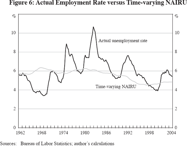
The TVN series associated with our basic inflation equation for the PCE deflator does not fall below 5.6 per cent, or rise above 6.3 per cent, over the period between 1962 and 1988. However, beginning in the late 1980s, the TVN drifts downwards until it reaches 4.5 per cent in 1998, and then it gradually rises to a final value of 4.9 per cent in the December quarter 2004. Thus we concur with the general consensus that the TVN is currently roughly in the vicinity of 5.0 per cent, but the TVN plotted in Figure 6 is distinctly lower over the 1996–2000 period than the previous published series displayed for the PCE deflator in Gordon (1998), which reached a minimum value of 5.1 per cent in mid 1998, in contrast to the mid-1998 value of 4.5 per cent shown in Figure 6.
4.3 The inflation equation: estimated coefficients and simulation performance
Table 5 displays the estimated coefficients for the model's Equation (2) for the GDP and PCE deflators. The sum of coefficients on the lagged inflation terms is always very close to unity, as in previous research.[18] The sum of the unemployment gap variables is around −0.6, which is consistent with a stylised fact first noticed in the 1960s that the slope of the short-run Phillips curve is about minus one-half. The consistency of our current results with this long-standing stylised fact provides evidence of the stability of the slope of the Phillips curve over time.
Of the supply shocks, the change in the relative import price and relative food-energy effect are consistently significant in both columns, with plausibly sized positive coefficients. The coefficient on the relative price of non-food non-oil imports is 0.11 in the GDP deflator equation and 0.07 in the PCE deflator equation. The PCE coefficient of 0.07 is about half of the 14 per cent share of imports in nominal GDP. We would have expected the import price coefficient to be smaller for the GDP deflator than for the PCE deflator, rather than the reverse, since imports are excluded from GDP but included in consumption. As expected, the coefficients on the food-energy variable are much higher in the equation for the PCE deflator than for the GDP deflator, because imported energy is a part of consumption, but not part of GDP (although energy products, the prices of which are determined on global markets, form some part of GDP). The coefficient on the medical care effect is close to unity for both deflators. The coefficients for the Nixon control variables are highly significant, have the expected signs, and are of similar magnitude to those in past research.
While most papers presenting time-series regression results display coefficients, significance levels, and summary statistics, few go beyond that and display results of dynamic simulations. Yet the performance of the inflation equation is driven in large part by the role of the lagged dependent variable terms, making dynamic simulations the preferable method for testing. To run such simulations, the sample period is truncated 10 years before the end of the full sample period, and the coefficients estimated from the sample through 1994 are used to simulate the performance of the equation for 1995 to 2004, generating the lagged dependent variables endogenously. Since the simulation has no information on the actual value of the inflation rate, there is nothing to keep the simulated inflation rate from drifting far away from the actual rate. The bottom of Table 5 displays results of this dynamic simulation. Two statistics on simulation errors are provided, the mean error (ME) and the root mean-squared error (RMSE). The simulated values of inflation are extremely close to the actual values, with a mean error over 40 quarters of only −0.13 per cent for the GDP deflator equation and a minuscule −0.05 per cent for the PCE deflator equation. For both equations, the RMSE of the simulations is substantially lower than the standard error of the estimate for the 1962–94 sample period. These simulation results are substantially better than those reported in Gordon (1998).
4.4 Long simulations with and without supply shocks
The aim of the rest of the paper is to assess the role of shocks and changes in monetary policy as causes of the marked reduction in business cycle volatility documented above. The role of supply shocks in the inflation equation can be examined by running alternative simulations that use the full set of supply-shock variables and alternatively set them to zero, either one at a time or together.[19] We use the full set of information provided by our data – the coefficients presented above in Table 5 – and run simulations of the inflation equation with the shock variables alternatively included and excluded.
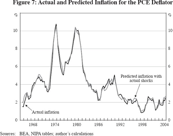
Figure 7 compares actual four-quarter changes in the PCE deflator with a dynamic simulation of the PCE deflator equation for the 160 quarters between 1965:Q1 and 2004:Q4, using the 1962–2004 period to estimate the coefficients as in Table 5. The dynamic simulation stays on track remarkably well over this long period. The same simulation is copied to Figure 8 and compared there with an alternative simulation that sets all supply-shock variables to zero. That is, inflation in this alternative simulation depends only on the simulated values of the lagged dependent variable terms plus the current and lagged values of the unemployment gap. Simulated inflation with no shocks remains roughly equal to the full-shock simulation through early 1973, and then stays consistently below the full-shock simulation by a very large amount for the next 30 years. Since the only variable driving a rise or fall in inflation is the unemployment gap, the severe recessions of 1974–75 and 1981–82 cause marked declines in the inflation rate, moving into negative territory in 1981, with a further fall in 1991–92 and a rise between 1995 and 2001. Notice that the difference between the two simulations narrows in the late 1990s, since the full-shock simulated value of inflation fails to rise between 1995 and 2001, due to the role of beneficial supply shocks, while the no-shock simulated value accelerates by about 2.5 percentage points.
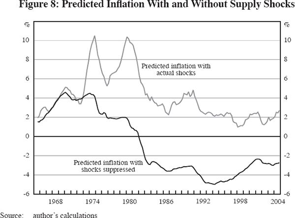
The prediction of deflation in Figure 8 highlights the problem of running a single-equation simulation in a multi-equation world. If there had been no adverse supply shocks in the 1970s, the recessions of 1974–75 and 1981–82 would have been much less severe or perhaps would not have happened at all. To develop a more realistic quantitative assessment of what would have happened without supply shocks in the inflation process, we need to develop a small macro model that allows us to trace the chain of causation from lower inflation volatility to lower output volatility, back to the behaviour of the unemployment gap term in the inflation equation.
5. Properties of a Four-equation Macro Model
There are numerous small macro models that could be used in this study, but none of them include the explicit treatment of supply shocks that is needed to adequately address the sources of inflation volatility. For instance, the ‘SVAR’ model used by Stock and Watson (2002, 2004) subsumes the role of supply shocks into the error term rather than modelling their role explicitly. The model developed in this paper starts with the inflation equation developed above and adds three extra equations. In order to evaluate the role of changing monetary policy responses, we add an equation for the nominal federal funds rate based on the Taylor rule, as in the SVAR model. Monetary policy can then influence output directly, and inflation indirectly, in the third equation, which makes the change in the output gap a function of lagged inflation and the change in the federal funds rate. Earlier we referred to this as a ‘three-equation’ model, but for convenience we add a fourth equation that links the unemployment gap (the demand variable in the inflation equation) to current and lagged values of the output gap. Using a notation that is consistent with the treatment of inflation above, the four-equation model can be written:
The symbol G stands for the level of the output or real GDP gap, that is, the log ratio of actual to natural real GDP, and ΔG stands for the first difference of the output gap. The Taylor rule equation for the federal funds rate includes the Fed's target for the real funds rate (T*), its target for the inflation rate (p*), the current and lagged deviations of the actual inflation rate from the inflation target, and current and lagged levels of the output gap. The output gap equation makes the change in the gap a function of one or more lags of the first difference of the inflation rate and of the change in the interest rate. Finally, the Okun's Law equation makes the level of the unemployment gap depend on the current value and one or more lags of the output gap.
The columns of Table 6 list the four dependent variables in the model, with the middle columns providing alternative sets of results for the interest rate equation. The choice of the three sub-intervals reflects apparent changes in Fed reactions – corresponding roughly to the three periods identified by Stock and Watson (2004, Table 5) – with breaks in 1979:Q3 (the start of the Volcker period) and in 1990:Q2 (the end of the period in which the Fed appeared to fight inflation aggressively while ignoring output deviations).
The second column of Table 6 shows coefficients in the inflation equation for the GDP deflator, which is identical to the equation already discussed in the first column of Table 5. The six middle columns show estimated Taylor rule equations for three periods split in 1979 and 1990. As a shorthand, we will refer to the three sub-intervals respectively as the ‘Burns’, ‘Volcker’, and ‘Greenspan’ responses. Let us first examine the first set of coefficients shown for each sub-interval, labelled ‘AR(1) Correction? No’. These coefficients show that before 1979, the Burns Fed ‘accommodated’ inflation, raising the nominal interest rate by less than half of any increase in the inflation rate, hence reducing the real interest rate and stimulating demand. After 1979, the inflation response jumped from 0.45 to 1.46, so that the Volcker Fed raised the nominal federal funds rate more than the increase of inflation above its target rather than less. The Greenspan Fed continued to respond aggressively to higher inflation, but also responded aggressively to the output gap, raising the nominal federal funds rate by almost a full percentage point in response to a positive output gap of 1 per cent. These coefficients reflect the widespread impression that the Greenspan Fed combined the best of both worlds, aggressively fighting inflation while also vigorously working to stabilise the output gap. Indeed, these coefficients for the Greenspan Fed correspond very closely to those for several alternative models surveyed by Stock and Watson (2004, Table 5, p 24).
However, this consensus conclusion is flawed by the extreme degree of positive serial correlation evident in the interest rate equation, especially for the Greenspan interval. To summarise what follows, the Burns and Volcker coefficients survive a serial correlation correction with their Taylor rule coefficients essentially intact, but the Greenspan coefficients turn out to be fragile. Let us take a simple version of the interest rate Equation (5), with the fixed constant term and lagged effects suppressed:

where 
To correct for the serial correlation represented by the positive value of ρ, we estimate Equation (8) in the following alternative form:

To correct for serial correlation, the interest rate equation was re-estimated using ‘feasible general least squares’ (FGLS), a procedure which estimates the basic equation, then regresses the residuals on their lag in order to find the autoregressive (ρ) coefficient, and then differences the terms based on that coefficient.[20] The alternative results are shown in the columns in Table 6 labelled ‘AR(1) Correction? Yes’. The correction makes little difference for the Volcker coefficients and slightly increases both the inflation and output gap responsiveness of the Burns reaction function. But the effect on the Greenspan coefficients is profound; the inflation response changes from an inflation-fighting 1.43 to an inflation-accommodating 0.57. The coefficient on the output gap falls by one-third, from 0.95 to 0.60. With the serial correlation correction, the Greenspan coefficients turn out to be almost identical to the Burns coefficients. In this sense, compared to pre-1979, the Greenspan era represents no improvement in monetary policy at all! All the model simulations displayed and discussed in the rest of this paper use the version of the interest rate equation that is corrected for serial correlation.
The ‘IS’ equation for the first difference of the output gap, shown in the second-last column of Table 6, shows an insignificant positive response to the first difference of the inflation rate, suggesting no direct feedback from a sharp increase of inflation to a sharp decrease in output, as might have been suggested by the economy's behaviour in the 1970s. The responses to changes in the nominal federal funds rate are of plausible size and highly significant; an increase in the funds rate by 100 basis points causes a decline in the output gap of 1 percentage point, with a long lag distributed over the next 10 quarters.[21] The final column in Table 6 exhibits the Okun's Law equation, showing that the unemployment gap responds to the output gap over the current and first two lagged quarters with a highly significant coefficient of −0.52.
5.1 Single-equation model simulations
The aim of building the model is to use it to decompose the sources of business cycle volatility. For this purpose we will focus on four different sources of volatility and its post-1983 reduction, namely the set of supply shocks included in the inflation equation; the error term in the interest rate equation; the error term in the output gap equation; and shifts in the parameters in the interest rate equation that reflect changes in Fed policy.[22] In this section we will examine the performance of each equation without model interactions; that is, each equation's predicted values are examined using actual historical values for the endogenous explanatory variables. Subsequently we will examine outcomes that feed back simulated values of the endogenous variables.
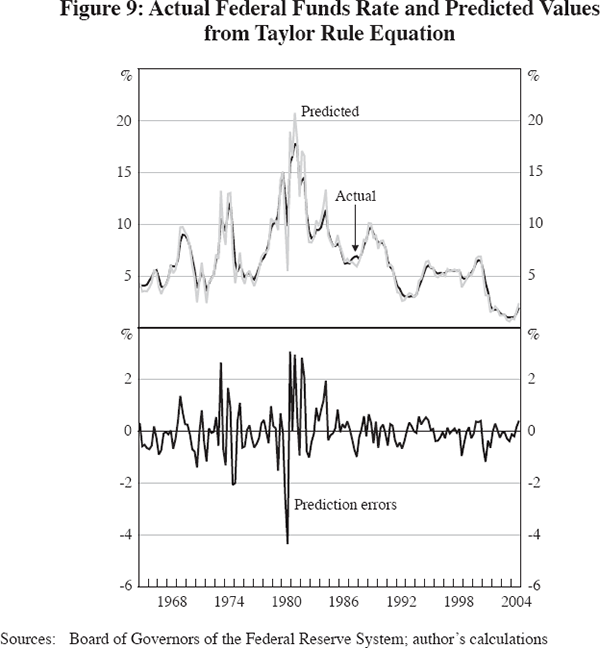
Having already examined the simulation performance and role of supply shocks in the inflation equation (see Figures 7 and 8), we now turn to the single-equation behaviour of the interest rate equation, taking its explanatory variables as exogenous. All the simulations in this paper assume that the inflation target (p*) in Equation (6) is 2.0 per cent and that the real interest rate target (T*) is 3.0 per cent. As in Table 6, the coefficients on inflation and the output gap are allowed to shift in 1979 and 1990. The fitted performance of the equation is extremely close to the actual values, as shown in the top frame of Figure 9, which is no surprise in light of the correction for serial correlation. Without that correction, the equation (using the estimated coefficients shown in Table 6 without the AR(1) correction) misses three aspects of interest rate behaviour after 1990. First, the Fed's ‘pre-emptive strike’ of raising the nominal federal funds rate sharply in 1994 is not captured by the equation. Second, the flatness of the rate between 1995 and 2000 is not captured; a Taylor rule would have increased the rate substantially more in response to the move of the output gap from negative to positive. Finally, and most important, the standard Taylor rule approach cannot explain why the Fed reduced rates so fast and kept them so low between 2001 and 2004.
The central topic of this paper is the reduced volatility of the output gap, as already examined in Figure 2. The predictive performance of the output gap equation is shown in Figure 10. While the equation is estimated in first-difference form, the actual and predicted values of the first differences are converted back to the level of the output gap in Figure 10.[23] Clearly, the output gap has a life of its own that is not captured by the simple ‘IS’ equation. The output gap equation misses about half of the boom of the late 1960s and of 1973, and predicts a much smaller recession in 1974–75 than actually occurred. In contrast, the equation's predictions overstate the severity of the 1980–85 slump, fail to capture the output gap's rise above zero in the late 1980s, and then completely miss the dynamics of the 1990s. The economy is predicted to be stronger in the early 1990s than the late 1990s, and in response to the Fed's aggressive rate reductions between 2001 and 2004, the economy is predicted to be much stronger in the current decade than actually occurred.
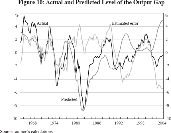
These errors in the output gap equation are not bad news for the model. Rather, they remind us that output depends on far more than movements back and forth along a fixed IS curve, as is implied by our model which makes changes in interest rates the only significant source of changes in the output gap. Obviously shifts in the IS curve matter as well, and it would take a much more complex model to capture the sources of these IS shifts. Missing from the predictions of the output gap equation in Figure 10 are such important events as Vietnam war spending in the late 1960s and the timing of the hi-tech investment boom of the late 1990s. In the full-model simulations discussed below we will explore the effects of suppressing the error term in the output equation.
Table 7 summarises the single-equation results that are plotted in Figures 8, 9 and 10. The top four lines calculate standard deviations of the actual values of the inflation rate, federal funds rate, and the level and first difference of the output gap. The reported standard deviations for the actual inflation rate and output gap are similar to those in the discussions of Figures 2 and 3 above, with a decline in the standard deviation of the output gap of more than half after 1983, and a decline in the standard deviation of the inflation rate by almost 60 per cent. In contrast, the volatility of the interest rate declined by much less – about 30 per cent.
| 1965–1983 | 1984–2004 | Ratio of 1984–2004 to 1965–1983 (per cent) |
|
|---|---|---|---|
| Actual values | |||
| Inflation rate | 2.40 | 1.00 | 41.7 |
| Federal funds rate | 3.63 | 2.49 | 68.6 |
| Level of output gap | 3.52 | 1.56 | 44.3 |
| First difference of output gap | 1.10 | 0.54 | 49.1 |
| Simulation results | |||
| Simulated inflation | 2.31 | 0.74 | 32.0 |
| Simulated inflation without supply shocks | 1.51 | 0.54 | 35.8 |
| Contribution of supply shocks | 2.57 | 0.67 | 26.1 |
| Predicted federal funds rate with interest error | 3.63 | 2.49 | 68.6 |
| Predicted federal funds rate without interest error | 3.51 | 2.33 | 66.4 |
| Predicted first difference of output gap with output error | 1.10 | 0.54 | 49.1 |
| Predicted first difference of output gap without output error | 0.53 | 0.31 | 58.5 |
|
Source: author's calculations |
|||
How well do the simulations (for the inflation equation) and predicted values (for the other equations) replicate the decline in the standard deviations of the actual variables? Simulated inflation falls by 68 per cent, even more than the actual value, and simulated inflation declines substantially whether supply shocks are included or excluded. However, as we have seen in Figure 8 above, much of the pre-1984 inflation volatility in the ‘no-shocks’ scenario is due to the role of deep recessions in forcing inflation into negative territory. A full understanding of the role of supply shocks requires us to unleash the full set of model interactions, since without supply shocks in the 1970s there would not have been the spikes of the interest rate in 1981–82, nor the deep recession of 1981–82.
The single-equation predictions for the federal funds rate differ from the other equations because the error term is so small, virtually eliminated by the serial correlation correction. The predicted value for the interest rate has a decline in its standard deviation of 32 per cent, identical to the actual decline. The output gap equation yields a predicted value (for the first difference of the gap) that has a decline in its standard deviation of 51 per cent, as compared to the actual decline of 55 per cent. Eliminating the error term in the output gap equation cuts the standard deviation by half before 1984 and by about 40 per cent after 1984, indicating that a reduction in the variance of the output error contributed to business cycle stabilisation after 1983.
5.2 Full-model simulations
To assess the role that supply shocks in the inflation equation played in reducing business cycle volatility, and the role of the error terms in the interest rate and output gap equations, we run full-model simulations with alternative shocks set equal to zero, one at a time and then all together. Table 8 contains five sections, one each for the standard deviation of inflation, the interest rate and the output gap, then the average value of inflation and the average absolute value of the output gap. Within each section there are five lines corresponding to the full-model simulations and alternative simulations that suppress the shocks one at a time and all together.
| 1965–1983 | 1984–2004 | Ratio of 1984–2004 to 1965–1983 (per cent) |
|
|---|---|---|---|
| Standard deviation of inflation
rate (percentage points) |
|||
| All shocks | 2.61 | 1.44 | 55.2 |
| No supply shocks | 0.60 | 0.67 | 111.7 |
| No output error | 2.11 | 0.99 | 46.9 |
| No interest error | 2.58 | 1.55 | 60.1 |
| No shocks | 0.00 | 0.00 | – |
| Standard deviation of fed funds
rate (percentage points) |
|||
| All shocks | 3.43 | 1.56 | 45.5 |
| No supply shocks | 1.72 | 1.43 | 83.1 |
| No output error | 1.66 | 0.59 | 35.5 |
| No interest error | 3.08 | 1.50 | 48.7 |
| No shocks | 0.00 | 0.00 | – |
| Standard deviation of output gap (percentage points) |
|||
| All shocks | 3.28 | 1.82 | 55.5 |
| No supply shocks | 1.89 | 1.94 | 102.6 |
| No output error | 1.06 | 0.33 | 31.1 |
| No interest error | 3.12 | 1.88 | 60.3 |
| No shocks | 0.00 | 0.00 | – |
| Average inflation rate (per cent) |
|||
| All shocks | 5.48 | 2.86 | 52.2 |
| No supply shocks | 3.41 | 4.15 | 121.7 |
| No output error | 3.23 | 1.31 | 40.6 |
| No interest error | 5.40 | 2.82 | 52.2 |
| No shocks | 2.00 | 2.00 | 100.0 |
| Average absolute value of output
gap (per cent) |
|||
| All shocks | 2.64 | 1.81 | 68.6 |
| No supply shocks | 1.77 | 1.69 | 95.5 |
| No output error | 1.28 | 0.84 | 65.6 |
| No interest error | 2.58 | 1.87 | 72.5 |
| No shocks | 0.00 | 0.00 | – |
|
Source: author's calculations |
|||
The contrast between the single-equation and full-model simulations can be seen by comparing Tables 7 and 8. This is summarised in Table 9, which shows the percentage ratio of the standard deviations for 1984–2004, relative to 1965–1983, using actual data for each of the three variables, the single-equation simulation values, and the full-model simulation values.[24]
| Four-quarter inflation rate |
Interest rate | Δ output gap | |
|---|---|---|---|
| Actual values | 41.7 | 68.6 | 49.1 |
| Single-equation simulations | 32.0 | 68.6 | 49.1 |
| Full-model simulations | 55.2 | 45.5 | 47.1 |
|
Source: author's calculations |
|||
Both the full-model simulations and the single-equation simulations include the exogenous effects of the supply-shock variables in the inflation equation, as well as the error terms in the interest rate and output gap equations. But they differ in that the former use endogenous model-generated values rather than actual values for the endogenous variables in each equation. While the model comes very close to duplicating the actual decline in the volatility of the output gap between the two periods, it understates the decline in the volatility of inflation and overstates the decline in the volatility of the interest rate.
Turning back to Table 8, we can now discuss the relative role of supply and demand shocks in explaining the model's simulated volatility. Because of the serial correlation correction, errors in the interest rate equation play no role in the explanation. While Table 8 displays the effect of suppressing the interest rate errors, they make virtually no difference and are not discussed further. We start with the alternative simulations for the inflation rate as described in the top section of Table 8. For the first period, suppressing the supply shocks eliminates almost 80 per cent of the standard deviation of inflation in the first period, while suppressing the output gap error eliminates about 20 per cent of the standard deviation of inflation in the first period. Suppressing supply shocks reduces the second period standard error by about half, and suppressing the output error reduces it by about one-third.
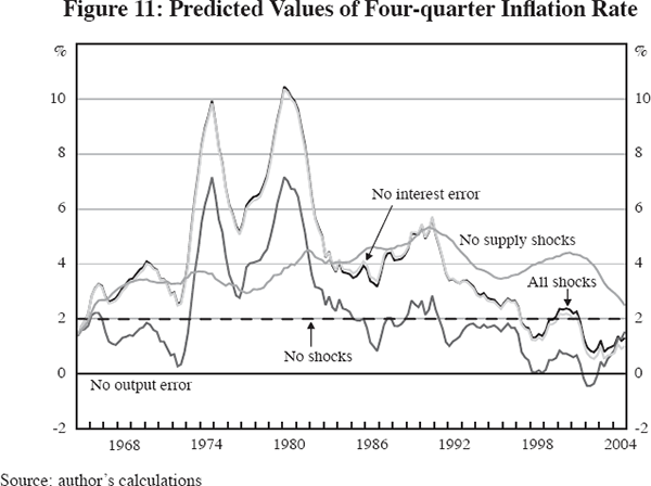
Figure 11 illustrates the role of supply shocks and the output error in explaining the behaviour of the inflation rate. The dark solid line shows the full model simulation, which is virtually identical to the single-equation simulations depicted in Figures 7 and 8. The interest error has little effect, but suppressing the output error reduces the inflation rate by a roughly constant 2 to 3 percentage points throughout the simulation period. Since the output equation cannot generate the excess demand of the late 1960s, without the output error the model forecasts less inflation throughout the full 40-year simulation period. What remains when the output error is suppressed represents the combined contribution of the supply shocks, causing a rise in inflation of 6 percentage points between 1972 and 1975, and a reversal in which inflation declined by about 5 percentage points between 1981 and 1984. Thus, ironically, the ‘Volcker disinflation’ that has usually been attributed to monetary policy should actually be credited in part to the reversal of supply shocks – not just the decline in the real price of oil, but also the effects of the dollar appreciation between 1980 and 1985.
Turning to the federal funds rate, Table 8 shows that in the first period, eliminating supply shocks reduces the standard deviation of the interest rate by half, as does eliminating the output error. In the second period, supply shocks have no impact on volatility, but suppressing the output error reduces the standard deviation of the interest rate by more than half. Thus much of the instability of the interest rate occurred through the effect of volatility of the output gap, generated by the output error directly, and indirectly by the effect of the output error in generating high inflation, rather than by monetary policy or supply shocks.
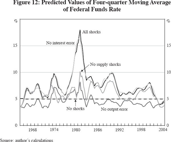
The simulations for the interest rate are displayed in Figure 12. Due to the correction for serial correlation, suppressing the model's own-equation interest rate errors makes virtually no difference. Compared to the basic model simulation, suppressing the supply shocks makes a big difference in holding down the interest rate between 1974 and 1985, but after 1985 this reduces the interest rate by only about 1 percentage point. Suppression of the output error also makes a big difference in reducing the interest rate throughout the 40-year simulation period, and particularly between 1977 and 1992. Recall that eliminating the output error works directly through the output gap term in the interest rate equation and indirectly though the effect of a lower output gap in reducing the inflation rate, and hence reducing the interest rate through the inflation term in the interest rate equation.
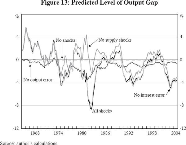
The next section of Table 8 tells a simple story, in which more than two-thirds of of the volatility of the output gap in the first period was caused by the output error and more than 80 per cent in the second period. Suppressing the supply shocks eliminates more than 40 per cent of the output gap volatility in the first period, but none in the second period. Figure 13 displays alternative simulations of the output gap. Suppressing the supply shocks converts the double recessions of 1975 and 1981–82 into a long period of prosperity, with the output gap bouncing around between 4 per cent and −2 per cent over the entire 1975–92 period. Suppressing the output error dampens fluctuations in the output gap but still leaves the economy vulnerable to the effects of supply shocks, particularly between 1975 and 1985 when a decade-long recession would have occurred. With no output error, the output gap in Figure 13 would have been very close to zero throughout 1987–2004.
While this paper is about the reduction in business cycle volatility, particularly about the post-1983 reduction in the standard deviation of inflation and the output gap, the Fed's objective as captured in the model's interest rate equation is not the standard deviation of the inflation rate but rather its average value. As for the output gap, the Fed's goal is for the output gap to be zero, and hence to minimise the average absolute value of the output gap. The bottom two sections of Table 8 report the effect of shocks on these two central objectives of Fed policy.
Suppressing the supply shocks and the output error would each have reduced the inflation rate by 2 percentage points, or about 40 per cent in the first period. In the second period, suppressing the supply shocks actually raises the inflation rate by more than 1 percentage point, since on balance during the second period the supply shocks were ‘beneficial’ rather than ‘adverse’. In contrast, suppressing the output error in the second period eliminates more than half of the inflation simulated by the full model. In the first period, suppressing the supply shocks eliminates one-third of the average absolute value of the output gap, whereas suppressing the output error eliminates slightly more than one-half. In the second period, suppressing the supply shocks has little effect on the output gap, but suppressing the output error reduces its average absolute value by more than half.
Overall, both the supply shocks and the output error contributed to the high volatility of inflation and the output gap before 1983, as well as to the high average value of inflation and the high average absolute value of the output gap. Suppressing the supply shocks makes the economy's behaviour in the first period similar to its behaviour in the second period, thus eliminating the puzzle of reduced volatility, and in fact suppressing the supply shocks makes average inflation in the second period higher than in the first period. Suppressing the output error makes the economy more stable and inflation lower in both periods. Without the output error, the output gap would have been much smaller and less volatile in both periods, and without the output error we still would have had a puzzle of improved post-1983 volatility that would have been resolved by the role of the supply shocks.
5.3 The role of changes in monetary policy
As shown in Table 6 above, the Fed's response to inflation and the output gap shifted over the three periods where breaks are allowed; 1960–79 (‘Burns’), 1979–90 (‘Volcker’), and 1990–2004 (‘Greenspan’). The big shift from Burns to Volcker was an increase in the response coefficient of the nominal federal funds rate to an increase of the inflation rate (relative to the 2.0 per cent target), from well below unity to well above unity (that is, from a policy of inflation accommodation to a policy of inflation fighting). The Volcker Fed cared only about fighting inflation and placed no weight at all on reducing the output gap. After 1990, under Greenspan, inflation fighting remained, but the response to the output gap increased from zero to nearly unity, as is consistent with the Fed's aggressive rate reductions from 1991 to 1993 and in 2001–02. However, as we have seen in Table 6, the estimated coefficients for the Greenspan period are tainted by positive serial correlation. When a serial correlation correction is applied, Greenspan's credentials as an inflation fighter disappear, and the Greenspan coefficients emerge looking just like the Burns coefficients.
The difference made by these shifts in Fed policy is shown in Figure 14, which plots four alternative paths of the output gap; all these full-model simulations include the output error and all use the coefficients from Table 6 that are corrected for serial correlation. The dark solid line labelled ‘split sample’ allows the Taylor rule coefficients to shift across the three periods. The other lines force the coefficients for a particular sub-interval to apply to the full 40-year simulation period. Since the Volcker coefficients do not respond at all to output but respond strongly to inflation, it is not surprising that the Volcker coefficients imply deeper recessions in 1971 and especially in 1975–76. Since this aggressive early response to inflation would have moderated inflation, a smaller recession in 1981–82 is implied. Also, the Volcker coefficients, by not responding to the positive output gap from 1998 to 2001, would have allowed the output gap to go higher. The Burns coefficients are not distinguishable on the chart before 1979, since their effect is the same as the ‘split sample’ line. After 1979, the less aggressive response to inflation would have resulted in a milder recession in the early 1980s. The Greenspan coefficients yield roughly the same path as the Burns coefficients, with shallower recessions in both 1975 and 1981–82 than the Volcker coefficients.
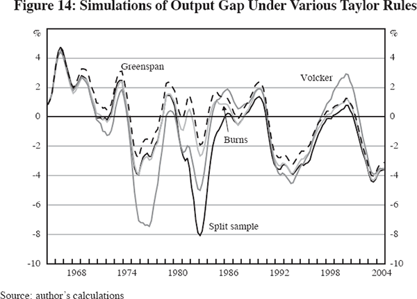
The simulation results from Figure 14 are summarised in Table 10. The top section shows that if the Volcker coefficients had been in effect before 1979, the volatility of inflation would have been reduced by about 20 per cent in both the first and second periods. The Greenspan coefficients would actually have made the volatility of inflation slightly higher in the first period, albeit lower in the second period. The next section shows that the Burns and Greenspan coefficients would have reduced the pre-1984 volatility of interest rates by more than half, and even the Volcker coefficients would have reduced interest rate volatility somewhat, by fighting inflation earlier and making the peak interest rates of 1980–81 unnecessary.
| 1965–1983 | 1984–2004 | Ratio of 1984–2004 to 1965–1983 (per cent) |
|
|---|---|---|---|
| Standard deviation of inflation
rate (percentage points) |
|||
| Split-sample coefficients | 2.61 | 1.44 | 55.2 |
| Burns | 2.62 | 1.26 | 48.1 |
| Volcker | 2.09 | 1.14 | 54.5 |
| Greenspan | 3.08 | 1.08 | 35.1 |
| Standard deviation of fed funds
rate (percentage points) |
|||
| Split-sample coefficients | 3.43 | 1.56 | 45.5 |
| Burns | 1.62 | 1.41 | 87.0 |
| Volcker | 2.73 | 1.49 | 54.6 |
| Greenspan | 1.56 | 1.39 | 89.1 |
| Standard deviation of output gap (percentage points) |
|||
| Split-sample coefficients | 3.28 | 1.82 | 55.5 |
| Burns | 2.25 | 1.98 | 88.0 |
| Volcker | 3.39 | 2.44 | 72.0 |
| Greenspan | 2.04 | 1.96 | 96.1 |
| Average inflation rate (per cent) |
|||
| Split-sample coefficients | 5.48 | 2.87 | 52.4 |
| Burns | 5.63 | 5.53 | 98.2 |
| Volcker | 4.44 | 2.81 | 63.3 |
| Greenspan | 6.53 | 7.92 | 121.3 |
| Average absolute value of output
gap (per cent) |
|||
| Split-sample coefficients | 2.64 | 1.91 | 72.3 |
| Burns | 1.90 | 1.78 | 93.7 |
| Volcker | 2.78 | 2.15 | 77.3 |
| Greenspan | 1.94 | 1.72 | 88.7 |
|
Source: author's calculations |
|||
Compared to the Volcker and split-sample outcomes, either the Burns or Greenspan coefficients would have reduced the standard deviation of the output gap in the first period by about one-third, as well as the average absolute value of the output gap (bottom section of Table 10). However, this improved performance on output volatility would have come at a cost of much higher inflation than the Volcker policy responses. In fact, by failing to fight inflation aggressively, the Greenspan coefficients would have yielded post-1983 average inflation of almost 8 per cent per year as compared to the 2.9 per cent average yielded by the split-sample policies and 2.8 per cent average yielded by the Volcker policies.
Which set of policies was ‘best’? There is no answer to that question without placing welfare weights on the average rate of inflation as compared to the average absolute value of the output gap. If what counts is the economy's performance in the long run, then the Volcker policies win the contest compared to the Burns or Greenspan policies. Consider the contrast between the Volcker and Greenspan policies. The Volcker response achieved 2 percentage points lower inflation before 1984 at the cost of 1 extra percentage point of the average absolute value of the output gap, the classic inflation-output trade-off. It is after 1984 that the pay-off from the Volcker policies becomes evident, with a full 5 percentage points less inflation than the Greenspan policies at the cost of only 0.4 of a percentage point higher average absolute output gap.
Much of the long-run benefit of the Volcker inflation-fighting policies occurred through the creation of a large recession in 1975. Would the verdict on the policies change if our simulations were to begin in 1979 instead of 1965, thus preventing the Volcker policies from having a counterfactual ‘head start’? Table 11 is laid out as per Table 10, showing the effects of the alternative monetary policy reaction functions in simulations that cover 1979–2004 in the first column and 1990–2004 in the second column. For the simulations starting in 1979, the Volcker policies achieve an average reduction of the inflation rate of 2 percentage points, at the cost of an average absolute output gap that is 0.7 of a percentage point higher. There is little difference between the policies in the simulations that begin in 1990.
| Simulation starts in 1979:Q3 | Simulation starts in 1990:Q3 | |
|---|---|---|
| Standard deviation of inflation
rate (percentage points) |
||
| Burns | 1.68 | 2.07 |
| Volcker | 2.17 | 2.21 |
| Greenspan | 1.77 | 2.14 |
| Standard deviation of fed funds
rate (percentage points) |
||
| Burns | 1.64 | 3.26 |
| Volcker | 2.93 | 3.17 |
| Greenspan | 1.69 | 3.18 |
| Standard deviation of output gap (percentage points) |
||
| Burns | 1.89 | 2.42 |
| Volcker | 2.52 | 2.69 |
| Greenspan | 1.81 | 2.35 |
| Average inflation rate (per cent) |
||
| Burns | 5.98 | 3.72 |
| Volcker | 3.87 | 3.47 |
| Greenspan | 5.81 | 3.60 |
| Average absolute value of output
gap (per cent) |
||
| Burns | 1.69 | 2.12 |
| Volcker | 2.38 | 2.47 |
| Greenspan | 1.65 | 2.09 |
|
Source: author's calculations |
||
5.4 The sacrifice ratio
If maintained throughout 1965–2004, the Volcker policies would have yielded an average inflation rate during 1984–2004 that would have been 5 percentage points lower than if the Greenspan policies had been maintained throughout 1965–2004. This hypothetical Volcker accomplishment was achieved at the cost of much deeper recessions in 1975 and 1981–82 than under the hypothetical Greenspan policies. A standard way to measure this trade-off is the ‘sacrifice ratio’, defined as the cumulative decline in output divided by the permanent fall in the rate of inflation. In the simulations in Table 11 that start in 1979:Q3, the Volcker policies would have delivered a cumulative annual output gap 15.2 percentage points lower (that is, more negative) than the Greenspan policies over the simulation through 1985:Q4, to achieve an inflation rate exactly 2.0 percentage points lower in the December quarter 1984 (and on average 2.0 points lower between 1986 and 1990). This yields a sacrifice ratio of 15.2/2, or 7.6, much higher than casual calculations of the sacrifice ratio observed in the actual data. For instance, the full-model simulation achieves a reduction in the four-quarter-ended inflation rate from 9.9 per cent in 1980 to 3.9 per cent in 1985, a decline of 6 percentage points, at the cost of a 20.7 cumulative percentage points negative output gap, for a sacrifice ratio of 3.5 (20.7/6.0).
What accounts for the difference between the Volcker and Greenspan sacrifice ratio of 7.6 and the apparent actual ratio of 3.5? Much of the disinflation of the early 1980s was achieved not just by the reduction in output and higher unemployment due to monetary policy, but also through a reversal of supply shocks, in particular the decline in oil prices from 1981 to 1986 and the decline in relative import prices associated with the 1980 to 1985 appreciation of the dollar. As shown in Figure 8 above, a single-equation simulation of the full inflation equation generates a reduction in the four-quarter-ended inflation rate of 8.1 percentage points between 1980:Q1 and 1986:Q4, compared to a reduction of 5.5 percentage points when the supply shocks are suppressed. In this sense about two-thirds of the disinflation of the early 1980s was achieved by tight money while the other one-third was due to a reversal of supply shocks. Admittedly, the supply shocks are partly endogenous, and some unknown fraction of the reversal of the supply shocks was in part a side-effect of tight monetary policy, especially that due to the appreciation of the dollar.
6. Conclusion
This paper investigates the sources of the widely noticed and discussed reduction in the volatility of American business cycles since the mid 1980s. Our analysis of reduced volatility emphasises the sharp decline in the standard deviation of changes in real GDP, of the output gap, and of the inflation rate. A preliminary examination of the data supports the conclusion of the previous literature that there was a break in US macroeconomic behaviour in 1983–84, after the end of the 1981–82 recession. Since then, expansions have been longer and recessions both less frequent and shallower. The aim of the paper is to determine the causes of the decline in volatility and allocate the decline among supply shocks, demand shocks, and improvements in monetary policy.
The first substantive section of the paper divides economic activity into the 11 major expenditure components of GDP. At this level of disaggregation about 80 per cent of the decline in output volatility can be attributed to lower volatility in the 11 individual components, and the remaining 20 per cent to a shift in spending shares toward more stable components, especially consumer services, and away from more volatile components, particularly investment in residential structures, inventory investment, and federal government spending. Taking covariances into account, these three sectors account for 50 per cent of the reduction in the average standard deviation of real GDP when the 1950–1983 and 1984–2004 intervals are compared, even though these three components accounted for only 17 per cent of nominal GDP in the first interval and 13 per cent in the second interval.
Up to this point the paper concludes that demand shocks played a major role in the reduction of volatility, particularly the reduced importance of federal military spending and the financial market reforms that helped to stabilise residential investment. In addition, information technology and other innovations helped reduce the importance of inventory fluctuations. Joining demand shocks as a disruptive force before 1984 were supply shocks that shifted the Phillips Curve primarily in an upward direction before 1981 and primarily in a downward direction after 1981. A simple piece of evidence that both demand and supply shocks mattered in the history of the American business cycle is provided in Figure 3, which shows that inflation and output volatility moved closely together between 1973 and 1988, but that there was ample output volatility in the 1950s and 1960s when inflation was relatively stable, and to a lesser extent there were episodes of sizeable output volatility after 1988, despite the relatively stable and quiescent inflation rate.
The paper develops a small macroeconomic model designed to measure the impact of supply shocks in the inflation equation and unidentified errors in the equations determining the federal funds rate and the output gap. The inflation equation included in the model builds on my own previous research, updating the so-called ‘mainstream’ model. Supply shocks included in the inflation equation include changes in the relative price of imports, the effect of changes in food-energy prices, the effect of changes in medical care prices, the effect of accelerations and decelerations in the productivity growth trend, and the effect of the Nixon-era price controls.
The inflation equation incorporates a natural rate of unemployment or ‘NAIRU’ that varies with time; its primary movement is a decline from about 6 per cent in the late 1980s to a minimum of about 4.5 per cent in the late 1990s, with an upward drift to about 4.8 per cent by 2004. Low inflation in the 1995–2004 period is explained in the model by the declining NAIRU, by accelerating productivity growth, and by the role of falling relative import prices between 1995 and 2002 and negative food-energy and medical care effects during particular sub-intervals. The inflation equation is tested not just by the usual criteria, that is, the significance and signs of coefficients and the goodness of fit, but also by dynamic simulations which generate the lagged dependent variables over long periods of time after the sample period; 40 quarters in the simulations reported here.
The inflation equation is joined by a second equation that determines the federal funds rate according to a standard Taylor rule specification that allows the responses of the funds rate to inflation and to the output gap to vary over three sub-intervals; 1960–79; 1979–90; and 1990–2004. The third equation relates changes in the output gap to past changes of the inflation rate and the funds rate. A symmetric analysis of shocks is developed. The specific supply-shock variables in the inflation equation can be included or set equal to zero. To develop a parallel treatment of shocks to interest rates and to the output gap, we allow the error term in those equations to be either included or excluded from model simulations.[25]
A very surprising finding in this paper is that the biggest driver of the business cycle, and of reduced post-1984 output volatility, is the error term in the output gap equation. Only about half of the standard deviation of actual output gap changes can be attributed to responses to inflation and interest rates; the remaining half is soaked up by the equation's error term. We interpret the output response to the interest rate as movements along a given IS curve, while the output errors represent shifts of the IS curve. Several important historical episodes, including the large and positive Vietnam-related output gap of the late 1960s, and the smaller but still positive ‘new-economy’ -related output gap of the late 1990s, are exogenous events and do not represent responses to monetary policy. The emphasis on the role of the output error term in the model is entirely consistent with, and complementary to, the decomposition analysis earlier in the paper that pointed to residential and inventory investment and to federal government spending as the main sources of output volatility prior to 1984.
The simulations of the full model provide important roles for both supply shocks in the inflation equation and for the error term in the output gap equation. About 80 per cent of inflation volatility and its reduction is explained by the supply-shock terms in the inflation equation, but a substantial 20 per cent is explained by the output error term – for example, the role of the otherwise unexplained late 1960s expansion in generating the acceleration of inflation from 1965 to 1971. Similarly, the explanation of interest rate volatility before 1984 is also shared between supply shocks and the output error. Supply shocks created inflation that generated an interest rate response, especially in the 1970s and early 1980s, while the output error made interest rates more volatile, both directly through the output gap term in the interest rate equation and indirectly through the inflation term.
The reduced volatility of business cycles, more than anything, refers to output volatility rather than inflation or interest rate volatility. In explaining why the standard deviation of the output gap was so high before 1984 and why it declined so much, more than half of the explanation in the model is provided by the error term in the output gap equation. Our final emphasis on ‘IS’ shifts as sources of output volatility before 1984 is consistent with the decomposition analysis that singled out residential and inventory investment, and federal spending, as the culprits lying behind these IS shifts.
Perhaps the most surprising result in this paper is that, when monetary policy is assessed solely in terms of alternative Taylor rule reaction functions and their effect, there was no difference between the ‘Greenspan’ monetary policy in effect in 1990–2004 and the ‘Burns’ reaction coefficients in effect in 1960–79. Only the ‘Volcker’ reaction coefficients in effect during 1979–90 represented a substantial departure. Previous impressions that the Greenspan reaction function represented a desirable combination of aggressive fighting against both inflation and the output gap are based on statistical estimates plagued by positive serial correlation. When a serial correlation correction is applied, the Greenspan reaction to inflation drops from an inflation-fighting value well above unity to an inflation-accommodation value well below unity, and is little different from the Burns-era coefficient.
The model can be simulated to apply the Taylor rule reaction functions from the Burns, Volcker, and Greenspan eras to the entire 1965–2004 history. Here we encounter a classic inflation-output trade-off. Applying the Volcker inflation-fighting coefficients throughout the 1965–2004 period, in contrast to applying the Greenspan coefficients to the full period, would have yielded a permanent reduction in the post-1984 inflation rate of 5 percentage points, at the cost of much weaker output over most of the 1974–84 period. The sacrifice ratio calculated for the period 1980–85 from the differences between the outcomes of the Volcker and Greenspan policies is 7.6, compared to a sacrifice ratio of 3.5 in the actual data. The paper attributes this difference to the reversal of adverse supply shocks during the 1981–85 interval.
Which monetary policy was ‘best’? The answer depends on the time period in question and the length of the time horizon. A Volcker-like anti-inflation reaction function introduced in 1965 would have worsened output volatility but yielded much lower long-run inflation than a hypothetical Greenspan-like policy introduced in 1965. However, a ‘split’ policy based on the actual historical succession of reaction functions, with Burns ceding to Volcker in 1979 and Volcker ceding to Greenspan in 1990, would have achieved the same long-run post-1984 inflation and output gap outcomes as a pure Volcker policy.
Numerous qualifications and caveats are warranted. The Greenspan policies may have the same statistical reaction function as the Burns policies but are better in ways that the simple interest rate equation cannot capture, including faster reactions (the pre-emptive strike against inflation in 1994 and the sharp interest rate cuts in 2001–02). At a deeper level, the reason the Greenspan reaction function shows a low ‘accommodative’ response to inflation is that there was no inflation to be fought against, thanks to the beneficial set of supply shocks in operation in the late 1990s. With adverse instead of beneficial shocks, the Greenspan reaction function might have looked much like Volcker's. Finally, the treatment of all supply-shock terms in the inflation equation as exogenous needs to be qualified. Changes in the relative price of imports, and to a lesser extent changes in oil prices, reflect exchange rate movements that respond to monetary policy. We conclude that a reversal of supply shocks played an important role in the disinflation of the early 1980s and subsequent stabilisation of output, but that reversal was itself in part a response to the Volcker monetary policies.
Footnotes
I am grateful to Ian Dew-Becker and Chris Taylor for inspired research assistance, extended through many evenings and several weekends, and to Dan Sichel, Kevin Stiroh, and Mark Watson for discussions and references. [1]
Star-studded? An alphabetical list of last names of a subset of authors and discussants will suffice: Baily, Barro, Bernanke, Blanchard, Blinder, Deaton, DeLong, Dornbusch, Eckstein, Eisner, Fischer, Grossman, Hall, McCallum, Meltzer, Moore, Shiller, Sims, Sinai, Summers, Taylor, Temin, Watson and Zarnowitz. [2]
Citations for the premature view included the Bronfenbrenner (1969) volume Is the business cycle obsolete? Also cited was a remark by Paul Samuelson that ‘the NBER has worked itself out of one of its first jobs, namely, the business cycle’ (Zarnowitz 1972, p 167). [3]
The conference was held at the Dorado Beach Hotel, Puerto Rico, 22–25 March 1984, almost exactly at the moment when retrospective historical research has determined that the American business cycle experienced a sharp and permanent decline in volatility (see Figure 1). [4]
This result does not deny that monetary policy might have improved in a broader sense, with better communication and transparency and credibility acquired from the pre-1990 fight against inflation. [5]
We date the transition between the Volcker and Greenspan eras as occurring in 1990 rather than 1987, because Fed behaviour in 1987–90 resembles the Volcker set of responses more than the Greenspan set of responses. [6]
In Table 2 the standard deviations are calculated from the four-quarter changes over the entire interval shown, in contrast to Figures 1–3 where, for graphical purposes, the standard deviation is calculated over rolling 20-quarter periods, and Table 1 where these are then averaged. [7]
The four-quarter change in inventory investment cannot be calculated, since inventory investment is frequently negative. As indicated in the note to Table 2, we took the first difference of inventory changes, divided by a 20-quarter moving average of inventory changes, and then calculated the standard deviation of the resulting ratio. One reason for the low value of the standard deviation in both periods is that much of the volatility of inventory changes appears in the 20-quarter moving average and disappears in the ratio. [8]
The 20 per cent figure is the percentage ratio of −0.6 on the bottom line in the third column to −2.9, the sum of the numbers on the bottom line in the second and third columns. [9]
A detailed analysis of the role of financial innovations in achieving the reduced volatility of residential housing and consumption spending is provided by Dynan, Elmendorf and Sichel (2005). [10]
As shown in Table 6, the model contains a fourth equation that translates the output gap into the unemployment gap. This fourth equation plays no essential role in the analysis and could easily be substituted out of the model. [11]
The ‘25-year’ interval refers to the conference at which the 1982 paper was given in roughly its final form, held at Brookings Institution in November, 1980. [12]
The work of Staiger, Stock and Watson (1997, 2001) is included within the label ‘mainstream approach’. [13]
Note, in particular, that lower-case p in this paper represents the first difference of the log of the price level, not the price level itself. [14]
While the estimated sum of the coefficients on lagged inflation is usually roughly equal to unity, that sum must be constrained to be exactly unity for a meaningful ‘natural rate’ of the demand variable to be calculated. [15]
The relative import price variable is defined as the rate of change of the non-food non-oil import deflator minus the rate of change of the dependent variable (GDP deflator or PCE deflator). The relative food-energy variable is defined as the difference between the rates of change of the overall PCE deflator and the ‘core’ PCE deflator. The Nixon-control variables remain the same as originally specified in Gordon (1982). The medical care variable is defined in the same way as the food-energy variable, that is, as the difference between the inflation rate of the deflator for PCE or GDP, and the inflation rate for that deflator when medical care spending is deducted from total PCE or GDP. The productivity trend is a Hodrick-Prescott filter (using 6,400 as the smoothness parameter) minus a six-year moving average of the same H-P trend. The only changes from the previous published paper on this approach (Gordon 1998) is the introduction of the medical care variable and the productivity trend variable (see Eller and Gordon 2003). [16]
Namely, the import variable is the change in the relative price of imports, which reaches a peak of about 12 per cent in 1974–75. The food-energy variable is not the relative price of food and energy, but rather the difference between the growth rates of the PCE deflator including and excluding food and energy, and this variable peaks at 3.2 per cent in 1974–75. [17]
The inclusion of lags 13–24 (years 4 through 6) is strongly significant in an exclusion test. As stated in the notes to Table 5, we conserve on degrees of freedom by including six successive four-quarter moving averages of the lagged dependent variable at lags 1, 5, 9, 13, 17, and 21, rather than including all 24 lags separately. [18]
We cannot use the technique of truncating the sample period, as in the previous section, because we are particularly interested in the adverse supply shocks of the 1970s, and a simulation based on an equation truncated at, say, 1973 would have too little information and degrees of freedom to estimate coefficients on the supply-shock effects. [19]
I am grateful to my research assistant Ian Dew-Becker for noticing the serial correlation problem in the Greenspan equation and implementing the FGLS procedure to fix it. [20]
The current and first lags of the interest rate are omitted in the output gap equation because of simultaneity; in the short run, changes in output and interest rates tend to be positively correlated as ‘IS shifts’ move the economy along the ‘LM curve’. [21]
No attention is paid to errors in the Okun's Law equation, which is viewed here as a purely mechanical bridge between the output and unemployment gaps. [22]
The errors in the first-difference equation are translated into errors in the level of the output gap by forcing the level errors to have a mean of zero over the 1965–2004 period. [23]
The middle section of Table 8 displays the standard deviation of the output gap; Table 9 refers to the standard deviation of the first difference of the output gap as in Table 7. [24]
The model includes a fourth equation, a simple Okun's Law relation to create a bridge between the unemployment gap included in the inflation equation and the output gap. [25]
References
Blanchard OJ and J Simon (2001), ‘The long and large decline in U.S. output volatility’, Brookings Papers on Economic Activity, 1, pp 135–164.
Bronfenbrenner M (ed) (1969), Is the business cycle obsolete?, New York, Wiley-Interscience.
Burns AF (1947), Stepping stones towards the future, Annual Report 27, NBER, New York.
Burns AF (1960), ‘Progress towards economic stability’, American Economic Review, 50(1), pp 1–19.
Dynan KE, DW Elmendorf and DE Sichel (2005), ‘Can financial innovation explain the reduced volatility of economic activity?’, paper presented at the Carnegie-Rochester Conference Series on Public Policy (Financial Innovation, Risk and Fragility), University of Rochester, 15–16 April.
Eller JW and RJ Gordon (2003), ‘Nesting the new Keynesian Phillips Curve within the mainstream model of U.S. inflation dynamics’, paper presented at CEPR Conference on ‘The Phillips Curve Revisited’, Berlin, 5–6 June.
Gordon RJ (1975), ‘Alternative responses of policy to external supply shocks’, Brookings Papers on Economic Activity, 1, pp 183–206.
Gordon RJ (1977), ‘Can the inflation of the 1970s be explained?’, Brookings Papers on Economic Activity, 1, pp 253–277.
Gordon RJ (1982), ‘Inflation, flexible exchange rates, and the natural rate of unemployment’, in MN Baily (ed), Workers, jobs, and inflation, Brookings Institution, Washington DC, pp 88–152.
Gordon RJ (ed) (1986), The American business cycle: continuity and change, Studies in Business Cycles, Vol 25, NBER, Chicago.
Gordon RJ (1998), ‘Foundations of the Goldilocks economy: supply shocks and the time-varying NAIRU’, Brookings Papers on Economic Activity, 2, pp 297–333.
Gordon RJ (2003), ‘Exploding productivity growth: context, causes, and implications’, Brookings Papers on Economic Activity, 2, pp 207–279.
Gordon RJ and SR King (1982), ‘The output cost of disinflation in traditional and vector autoregressive models’, Brookings Papers on Economic Activity, 1, pp 205–242.
Staiger D, JH Stock and MW Watson (1997), ‘The NAIRU, unemployment and monetary policy’, Journal of Economic Perspectives, 11(1), pp 33–49.
Staiger D, JH Stock and MW Watson (2001), ‘Prices, wages and the U.S. NAIRU in the 1990s’, in AB Krueger and RM Solow (eds), The roaring nineties: can full employment be sustained?, The Russell Sage Foundation and The Century Foundation Press, New York, pp 3–60.
Stock JH and MW Watson (2002), ‘Has the business cycle changed and why?’, in M Gertler and K Rogoff (eds), NBER macroeconomics annual 2002, MIT Press, Cambridge, pp 159–218.
Stock JH and MW Watson (2004), ‘Has the business cycle changed? Evidence and explanations’, in Monetary policy and uncertainty: adapting to a changing economy, A Symposium Sponsored by the Federal Reserve Bank of Kansas City, Federal Reserve Bank of Kansas City, Kansas City, pp 9–56.
Zarnowitz V (1972), The business cycle today, Columbia University Press, New York.