RBA Annual Conference – 2005 When the US Sneezes, Do We Need to Catch a Cold? Historical and Future Linkages between the Australian and US Business Cycles Mark Crosby and Philip Bodman
Abstract
Many observers worry that when the economy of the United States sneezes, the rest of the world catches a cold. In the case of Australia, the linkage is usually seen to be particularly strong, with Australia's business cycle being much more correlated with the US cycle than most other OECD economies. In this paper we examine the relationship between the Australian and the US economy for the last 130 years. We argue that the very high post-war correlation between the Australian and US cycles is driven largely by the early 1980s and early 1990s recessions, and the associated high interest rates of these periods. With monetary policy now expected to achieve low inflation into the foreseeable future, we see no reason for the high correlation between the Australian and the US economies evident from 1980 to 2000 to continue into the next 20 years.
1. Introduction
In this paper we examine the linkages between the Australian and United States economies since 1870. It is common to hear the expression, ‘when the US sneezes, Australia catches a cold’.[1] From a policy-maker's perspective, understanding the historically high correlation between Australian and US cycles is critical. Is this correlation unavoidable, or is it avoidable through the right policy choices? Has policy caused this high correlation? Is this correlation simply coincidental? In this paper we argue that the historically high correlation between the two cycles is particular to the period from 1980 to 2000, and is driven largely by the similarity of monetary policy during this period. Looking into the future we do not anticipate the two cycles to be as highly synchronised as in the 1980s and 1990s.
The structure of our paper is as follows. In the next section we briefly discuss related literature, and review the evidence on the high degree of synchronisation between Australian and US cycles. Section 3 of the paper examines the evidence on the lack of synchronisation between the Australian and the US economies between 1870 and 1939, while Section 4 examines the post-war evidence on synchronisation patterns. In Section 5 we provide some tentative explanations for the changing correlation between Australian and US cycles in the post-war period, and the final section of the paper offers concluding comments.
2. Related Literature
The recent surge of research in the field of optimal currency areas has led to a number of papers that seek to describe and explain cross-country business cycle correlations, particularly among OECD countries. The desirability of a currency union depends in part on the extent to which participating countries' economies are synchronised. As a result, much effort has gone into trying to explain synchronisation, and also into trying to predict the impact that changes such as the formation of a currency union and greater trade integration have on business cycle synchronisation. Frankel and Rose (1998) argue that countries that have closer trade linkages tend to have more closely synchronised business cycles. On this basis they argue that steps that enhance economic and trade integration between countries are likely to lead to more synchronised cycles and therefore make currency unions more desirable. Similarly, Clark and van Wincoop (2001) find that states within the US are much more closely synchronised than countries within Europe, a result which they attribute mostly to closer trade linkages within the US as compared with European countries. Rose and Engel (2000) also find that countries in currency unions trade more, and have more highly synchronised business cycles than countries not in currency unions.
While the above papers suggest that trade is an important determinant of business cycle synchronisation, a number of authors have suggested that, once other determinants of synchronisation are properly controlled for, this effect is quite small. Imbs (2000, 2004) finds that this literature ignores structural similarity and financial specialisation, which he argues to be important factors in explaining synchronisation. Using a measure of similarity that depends on the shares of employment in each sector of the economy in each country, Imbs (2000) finds that structural similarity is able to explain much more of the cross-country variation in business cycle synchronisation within the OECD than trade. He also estimates that the rise in trade between 1963 and 1990 has caused a small increase in synchronisation, but that this has been more than offset by an increase in specialisation that has reduced synchronisation. In Imbs (2004) it is found that intra-industry trade has a sizeable effect on business cycle synchronisation, while inter-industry trade has only a small impact on synchronisation. Kose, Prasad and Terrones (2003) also find only limited evidence of trade increasing business cycle synchronisation. In addition, they find that business cycle co-movements have not changed significantly between the period from 1960 to 1980, and the period from 1981 to 1999. Heathcote and Perri (2003) also document changes in business cycle correlations with the US, and find that over the last 40 years the rest of the world has become less synchronised with the US.
Otto, Voss and Willard (2001) include measures of trade, similarity of economic structure, and financial and monetary policy linkages in their model of business cycle synchronisation for 17 OECD countries. They argue that most of the alternative transmission channels captured by structural variables act as proxies for trade, though there is some evidence that similar exchange rate behaviour can help explain synchronisation. They also argue that there is evidence that their basic model is misspecified (and the same is likely to be true of the models discussed above). In addition to trade, they find that country characteristics such as similarity of technological development, language and legal structures are important explanators of synchronisation. Crosby (2003) examines business cycle correlations in the Asia-Pacific region and finds that trade is a poor predictor of synchronisation, and synchronisation patterns are, in general, difficult to explain using any of the variables used to explain OECD correlations.
While there is debate over the statistical significance of trade and other factors in explaining synchronisation, it should be said that all of these studies find that trade is able to explain very little of the variability in business cycle correlations – R-squared values are typically around 0.2, and never above 0.4 in the many regressions estimated in the above papers.
The papers outlined above tend to take a cross-section approach to the examination of business cycle correlations. In this paper we narrow the focus to just the Australia–US correlation. Our approach is non-structural, but rather aims to document the facts regarding the Australia–US cycle correlation over time. In the penultimate section of the paper we provide some discussion on what has been driving the changing correlation patterns over time, and predict where these correlations may go in the future.
3. Historical Evidence on Australian–United States Synchronisation
In this section we examine the correlations between Australian and US GDP in the period 1870 to 1939. While there have no doubt been many fundamental changes in both economies subsequent to 1939, there are two reasons to examine the pre-war synchronisation patterns. Firstly, this period allows us to make some interesting observations relevant to the debate over whether structural similarities, trade intensity, or other factors are most important in synchronising business cycles. Secondly, there is little existing evidence on pre-war synchronisation, and documenting the facts regarding Australia's correlation patterns with other economies is of interest in its own sake.
We should note that there are some obvious difficulties in comparing pre-war economies given that the quality of the data and the methods used in its construction are not as consistent across countries as in the post-war era. It is also impossible to find data as detailed as those available today, and so we are forced to take a somewhat superficial approach when examining issues such as the structural similarity of the Australian and US economies. The data that we have used come from a variety of sources, including Maddison's (1995) estimates of real GDP, Meredith and Dyster (1999) for the Australian data, and Lee and Passell (1979) for the US data.
3.1 Basic features of the Australian and US economies prior to 1939
In Table 1 we document some basic facts about Australia, the US and the UK in the pre-1939 period. In 1870, agriculture's share of GDP was very similar in Australia and in the US, while the UK was much more reliant on mining and manufacturing. Over the next 60 years the US gradually shifted towards a greater reliance on mining and manufacturing, while Australia's share of agriculture, and mining and manufacturing in GDP remained remarkably stable. By 1930 agriculture was only 4.1 per cent of UK GDP, while the mining and manufacturing share was still significantly larger than in the US. These trends would lead us to expect that the Australian and US economies were somewhat synchronised in 1870, but became less so by 1930.
| 1870s | 1890s | 1910s | 1930s | ||
|---|---|---|---|---|---|
| Structural variables (per cent of GDP) |
|||||
| Australia(a) | Agriculture | 23.9 | 22.5 | 29.3 | 21.0 |
| Mining & manufacturing | 18.1 | 15.0 | 17.9 | 20.9 | |
| US(b) | Agriculture | 21.6 | 15.2 | 17.0 | 10.4 |
| Mining & manufacturing | 17.5 | 24.7 | 22.2 | 26.2 | |
| UK(c) | Agriculture | 14.2 | 8.6 | 6.0 | 4.1 |
| Mining & manufacturing | 38.1 | 38.4 | 37.0 | 40.2 | |
| Trade variables | |||||
| Exports (per cent of GDP) |
Australia(d) | 22.5 | 13.7 | 25.2 | 13.8 |
| US(e) | 6.2 | 6.5 | 4.8 | 4.2 | |
| Per cent of total exports |
Australia (wool)(f) | 37.0 | 65.2 | 38.0 | 33.0 |
| US (cotton)(g) | 47.8 | 28.3 | 24.2 | 14.9 | |
| Per cent of exports to UK |
Australia(f) | 60.9 | 68.8 | 47.0 | 46.2 |
| US(h) | 52.7 | 52.2 | 29.0 | 17.6 | |
| Terms of trade (1910 = 100) |
Australia(i) | 90.2 | 101.9 | 100.0 | 76.1 |
| US(j) | 79.7 | 91.4 | 100.0 | 123.0 | |
| (a) Butlin (1985). Agriculture includes pastoral and dairying. (b) Lee and Passell (1979, p 273). Data for the 1870s are the average for 1869–79; for the 1890s they are the 1889–99 average, while in the final column they are the 1919–40 average. The 1910s data are the 1904–13 average from United States Bureau of the Census (1975, p 238). (c) Mitchell (1988). Data are for 1871, 1891, 1907 and 1924. (d) Butlin (1962) and EconData DX database (e) United States Bureau of the Census (1975, p 887) (f) Butlin (1962, p 410), and Meredith and Dyster (1999, pp 63 and 137) (g) United States Bureau of the Census (1975, chapter U) (h) United States Bureau of the Census (1975, p 903) (i) Bambrick (1970) (j) Williamson (1964, p 262) |
|||||
A significant difference between the Australian and the US economies was in respect to the relative openness of the two countries. Australia's ratio of exports to GDP was quite variable, but was always much larger than the US equivalent. Interestingly, both countries were very exposed to a single export commodity in the early part of the period documented – wool in the case of Australia and cotton in the case of the US. Australia, however, remained reliant on wool throughout the period, while the US reliance on cotton fell from almost 50 per cent of exports to under 15 per cent. Both countries were also very reliant on the UK as a major trading partner. Once again, however, Australia's reliance persisted while US exports to the UK fell from 53 per cent of total exports to 18 per cent in 1930. The table also shows movements in the terms of trade – particularly notable is the dramatic fall in the terms of trade from 1910 to 1930 in Australia, illustrating the fact that the prices of the two countries' exports diverged during the inter-war period.
Overall, the data paint a picture of two economies that were quite similar in 1870 – economies with large agricultural sectors, reliant on the UK for trade concentrated around a small number of important exports. By 1930 these structural features remained intact for the Australian economy, while the US saw a halving of agriculture's share of GDP, along with a fall in the reliance on cotton and the UK in regard to exports.
3.2 Correlation patterns in the pre-war period
We use two basic approaches to examine synchronisation between the Australian and US economies pre-1939. Firstly, we document the correlation between GDP growth rates of the G7 countries plus Australia and NZ over different sub-periods prior to 1939. We also use the historical business cycle dating scheme from the National Bureau of Economic Research, along with some existing dates for business cycles in Australia, to compare cycles in the two countries.
Table 2 presents correlations between GDP growth rates in Australia and those in eight other countries between 1870 and 1939. The first era of globalisation, prior to World War I, was characterised by movements in Australia's GDP that were not closely related to any G7 country.[2] The highest contemporaneous correlation was 0.23 with NZ, and the correlations with the US and Canada were negative. Australia's similarity in structure to the US did not lead to synchronised cycles in this period, but it is also true that the strong trade linkages with the UK did not lead to synchronisation with that country.
| Canada | France | Germany | Italy | Japan | NZ | UK | US | |
|---|---|---|---|---|---|---|---|---|
| 1870–1913 | −0.09 | 0.08 | 0.22 | 0.08 | 0.19 | 0.23 | 0.17 | −0.16 |
| 1919–1939 | 0.02 | 0.13 | 0.52 | 0.07 | 0.20 | 0.26 | 0.07 | 0.17 |
| 1930–1939 | 0.51 | 0.47 | 0.63 | 0.47 | 0.48 | 0.70 | 0.81 | 0.49 |
|
Sources: authors' calculations, using Maddison (1995) |
||||||||
The inter-war pattern of correlations with Australia is a story of two correlation structures. In the 1920s, the Australian economy was again uncorrelated with the major economies and uncorrelated with NZ, so that the correlations for 1919–39 were only significantly different from zero in the case of Germany. The correlation with the US was positive but small, while the correlation with NZ was similar to that found prior to 1913. The correlations during the 1930s were positive and significantly different from zero for all countries, as they moved into recession together. For this period, there was a high correlation between Australian and US GDP growth, but the highest correlations were with NZ and the UK. (Later we examine the post-1945 data and also find that recessions tend to synchronise business cycles.) A small number of recessions experienced coincidentally across a large number of countries seems to be an important factor in understanding the cross-section data on business cycle correlations.
3.3 Recession dates prior to 1939
As well as utilising GDP data, it is informative to examine business cycle chronologies. These chronologies provide evidence on whether the timing of recessions is similar across countries – it is possible, for example, that GDP growth rates are correlated (or uncorrelated) but recessions are experienced at dissimilar (similar) times. The NBER chronology for the US provides dates for peaks and troughs beginning in 1857. We use this chronology for the US, and compare it to the Australian business cycle dates presented in Pagan (1996). (There is no official organisation that provides widely recognised business cycle dates in Australia prior to 1939, and Pagan simply provides a table of peak and trough dates for the classical cycle as gleaned from a variety of sources. The lack of consistency arising from taking dates from different sources is an issue here, but there is no other dating scheme available.) We also graph the years in which Australia's GDP growth was negative, along with negative growth years for the US.
Figure 1 shades each year for which the relevant country was in recession for any part of that year, using the NBER and Pagan dates (the dates provided for Australia are not as precise as the dates for the US in documenting which month or quarter was a peak or trough date, so this is a fair way to compare the available data). The figure illustrates two points very clearly. First, the US experienced a lot of years during which at least some time was spent in recession. If one takes the actual NBER dates, then for the period 1870 to 1900, 49 per cent of months are spent in the contraction phase of the business cycle. From 1900 to 1939 this percentage falls, but only to 42 per cent. Pagan (1996) lists only one recession in Australia in the 1870 to 1900 period, the severe recession of the 1890s, while there were seven recessions in the period from 1900 to 1939.
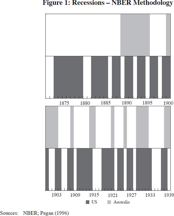
The second point is that the timing of recessions appears to be quite different, except that both countries are in recession in the 1890s and the 1930s.
Figure 2 shows the years for which GDP growth was negative in Australia and in the US. Australia experienced more years of negative growth than the US from 1870 to 1900, with both countries having the worst of it in the 1890s. The post-1900 period was dominated by the Depression, though overall the US had more years of negative growth from 1900 to 1939. The conclusion regarding synchronisation remains as above. Aside from the severe downturns of the 1890s and the 1930s, recessions in Australia and the US were generally not coincident.
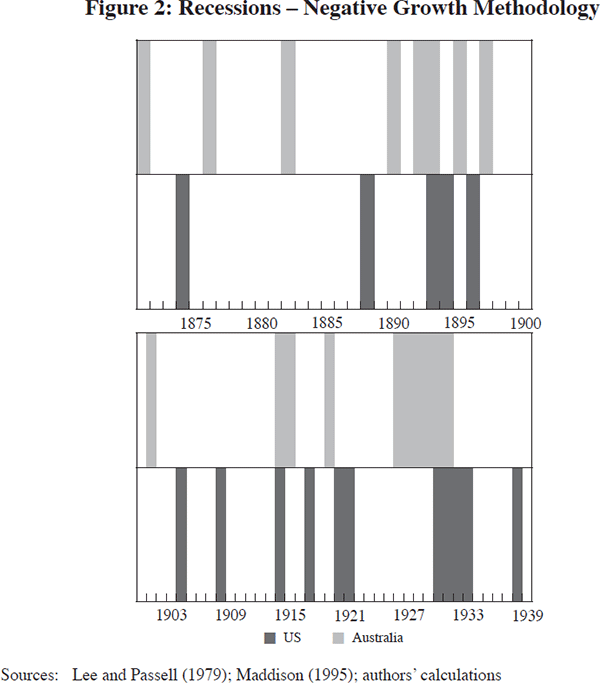
Overall this section illustrates quite clearly a couple of points. First, the Australian business cycle prior to 1939 was not particularly synchronised with the US (despite structural similarities that were quite evident in 1870) nor with other G7 economies. Second, Australia's connection with the economies of the rest of the world was restricted to the joint experience of two serious recessions.
4. The Post-war Experience
In this section we analyse the post-war relationship between Australian and US business cycles. We begin by examining the correlation between Australian cycles and cycles in G7 countries, using methods similar to those employed in the papers described in Section 2. We then characterise both the changing nature of Australian output growth and its evolving relationship with US output growth since the early 1960s. We find that the high correlation between Australian and US GDP appears from around the time of the first oil shock in the early 1970s.
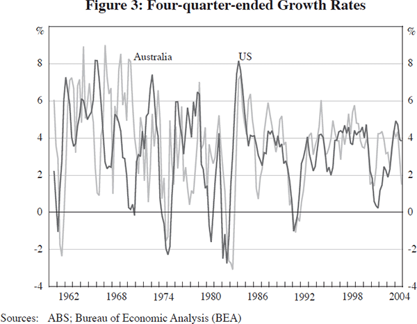
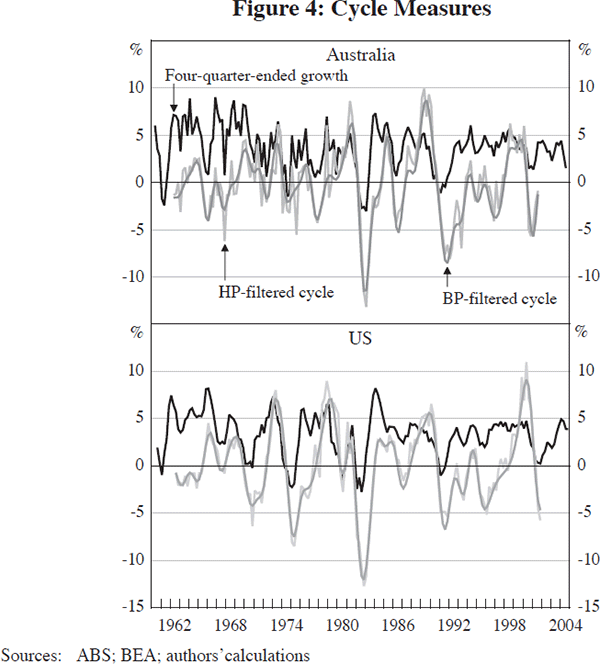
We focus our analysis in this section primarily on four-quarter-ended GDP growth rates for Australia and the US. Figure 3 provide a comparison between the two countries' growth rates, while Figure 4 compares the four-quarter-ended GDP growth rates to the levels data filtered using the Hodrick-Prescott filter and the Baxter-King band-pass filter. It can be seen that the filtered data are highly correlated with the four-quarter-ended data and we do not find any significant difference in our conclusions regarding synchronisation when we use the filtered data instead of the growth rate data.
4.1 Correlations between Australian cycles and G7 cycles
In this sub-section we provide some simple comparative evidence on the correlation of the Australian cycle with all of the G7 countries. Table 3 suggests that the Australian economy has become much more highly correlated with the English-speaking countries of the G7 in the 1980s and 1990s and more decoupled from the economies of Germany and Japan. In the table we also compute the correlations with Australia when dates in which Australia is in recession are excluded. We date recessions using either one of two rules; at least two quarters of negative growth, or by taking dates from the Economic Cycle Research Institute (ECRI), which dates recessions using a methodology similar to that employed by the NBER to date US cycles (see Tables 4 and 5 for the actual dates). Correlations between Australia and the other English-speaking countries are lower in the expansion phase of the business cycle than in the full sample. This is particularly true when the ECRI dated recessions are excluded. In particular, the Australia–US correlation drops from 0.34 to 0.12 when one examines only the dates when Australia is not in recession.
| Sample | US | Canada | Germany | France(a) | UK | Italy | Japan |
|---|---|---|---|---|---|---|---|
| 1961:Q1–1969:Q4 | −0.05 | −0.37 | 0.05 | – | 0.13 | −0.36 | 0.00 |
| 1970:Q1–1979:Q4 | 0.08 | 0.26 | 0.45 | – | 0.19 | 0.56 | 0.40 |
| 1980:Q1–1989:Q4 | 0.57 | 0.72 | 0.46 | 0.14 | 0.11 | 0.60 | 0.42 |
| 1990:Q1–1999:Q4 | 0.80 | 0.79 | −0.80 | 0.19 | 0.88 | 0.06 | −0.49 |
| 2000:Q1–2004:Q4 | 0.28 | 0.07 | −0.08 | −0.20 | 0.07 | −0.38 | −0.22 |
| 1961:Q1–1982:Q4 | 0.24 | 0.39 | 0.34 | – | 0.19 | 0.28 | 0.38 |
| 1983:Q1–2004:Q4 | 0.59 | 0.66 | −0.37 | 0.16 | 0.50 | 0.30 | −0.02 |
| 1992:Q1–2004:Q4 | 0.39 | 0.34 | −0.12 | 0.05 | 0.52 | −0.03 | −0.22 |
| 1961:Q1–2004:Q4 | 0.34 | 0.51 | 0.05 | 0.14 | 0.27 | 0.26 | 0.26 |
| Expansions only(b) | 0.12 | 0.30 | 0.21 | 0.05 | 0.19 | 0.25 | 0.31 |
| Expansions only(c) | 0.30 | 0.42 | 0.18 | 0.09 | 0.23 | 0.29 | 0.38 |
|
(a) Correlations with France begin in 1980:Q1. Sources: ECRI; NBER; authors' calculations |
|||||||
| Period | Peak (P)/ trough (T) |
Australia 1948– |
US 1948– |
Canada 1948– |
Germany 1950– |
France 1951– |
UK 1952– |
Italy 1956– |
Japan 1953– |
|---|---|---|---|---|---|---|---|---|---|
| 1948–50 | P | 11/48 | |||||||
| T | 10/49 | ||||||||
| 1951–52 | P | 6/51 | |||||||
| T | 9/52 | 8/52 | |||||||
| 1953–55 | P | 7/53 | 5/53 | ||||||
| T | 5/54 | 6/54 | 12/54 | ||||||
| 1956–59 | P | 12/55 | 8/57 | 10/56 | 11/57 | ||||
| T | 8/56 | 4/58 | 2/58 | 4/59 | |||||
| 1960–61 | P | 12/60 | 4/60 | ||||||
| T | 9/61 | 2/61 | |||||||
| 1962–66 | P | 3/66 | 1/64 | ||||||
| T | 3/65 | ||||||||
| 1967–68 | P | ||||||||
| T | 5/67 | ||||||||
| 1969–72 | P | 12/69 | 10/70 | ||||||
| T | 11/70 | 8/71 | |||||||
| 1973–76 | P | 6/74 | 11/73 | 8/73 | 7/74 | 9/74 | 4/74 | 11/73 | |
| T | 1/75 | 3/75 | 7/75 | 6/75 | 8/75 | 4/75 | 2/75 | ||
| 1976–80 | P | 1/80 | 8/79 | 6/79 | |||||
| T | 7/80 | 6/80 | |||||||
| 1980–83 | P | 6/82 | 7/81 | 4/81 | 1/80 | 4/82 | 5/80 | ||
| T | 5/83 | 11/82 | 11/82 | 10/82 | 5/81 | 5/83 | |||
| 1984–86 | P | ||||||||
| T | 12/84 | ||||||||
| 1987–89 | P | ||||||||
| T | |||||||||
| 1990–91 | P | 6/90 | 7/90 | 3/90 | 1/91 | 5/90 | |||
| T | 12/91 | 3/91 | |||||||
| 1992–94 | P | 2/92 | 2/92 | 4/92 | |||||
| T | 3/92 | 4/94 | 8/93 | 3/92 | 10/93 | 2/94 | |||
| 1995–99 | P | 3/97 | |||||||
| T | 7/99 | ||||||||
| 2000–04 | P | 3/01 | 1/01 | 8/00 | |||||
| T | 11/01 | 8/03 | 4/03 | ||||||
| Months in recession | 68 | 104 | 72 | 140 | 88 | 63 | 92 | 121 | |
| Fraction of time in recession |
0.099 | 0.152 | 0.105 | 0.212 | 0.136 | 0.099 | 0.156 | 0.194 | |
| No of recessions | 6 | 10 | 4 | 5 | 5 | 4 | 5 | 5 | |
| No of months jointly in recession with Australia |
– | 22 | 11 | 21 | 17 | 18 | 18 | 7 | |
|
Sources: ECRI; NBER |
|||||||||
| Period | Peak (P)/ trough (T) |
Australia 1960– |
US 1956– |
Canada 1956– |
Germany 1960– |
France 1970– |
UK 1956– |
Italy 1960– |
Japan 1956– |
|---|---|---|---|---|---|---|---|---|---|
| 1956–59 | P | 1/56 | |||||||
| T | 3/56 | ||||||||
| P | 3/57 | 3/57 | 1/57 | ||||||
| T | 1/58 | 1/58 | 4/57 | ||||||
| 1960–63 | P | 1/61 | 2/63 | 2/61 | |||||
| T | 4/61 | 1/63 | 4/61 | ||||||
| 1964–68 | P | 2/65 | 3/66 | 1/64 | |||||
| T | 1/66 | 2/67 | 4/64 | ||||||
| 1969–75 | P | 3/71 | 3/69 | 2/73 | 3/69 | ||||
| T | 1/72 | 1/70 | 1/74 | 1/70 | |||||
| P | 2/75 | 2/74 | 1/74 | 3/74 | 1/75 | 2/74 | |||
| T | 4/75 | 1/75 | 2/75 | 1/75 | 3/75 | 2/75 | |||
| 1976–78 | P | 2/77 | 1/77 | ||||||
| T | 4/77 | 3/77 | |||||||
| 1979–80 | P | 1/80 | 1/80 | 1/80 | 1/80 | 4/79 | |||
| T | 3/80 | 3/80 | 4/80 | 4/80 | |||||
| 1981–86 | P | 3/81 | 3/81 | 2/81 | 1/82 | 1/82 | |||
| T | 1/82 | 1/82 | 4/82 | 3/82 | 1/81 | 4/82 | |||
| P | 2/82 | ||||||||
| T | 1/83 | ||||||||
| 1987–91 | P | 4/90 | 3/90 | 1/90 | 2/90 | ||||
| T | 3/91 | 1/91 | 1/91 | 3/91 | |||||
| 1992–96 | P | 3/92 | 3/92 | 1/92 | 1/92 | ||||
| T | 2/93 | 3/93 | 4/92 | 3/92 | |||||
| P | 3/93 | ||||||||
| T | 1/94 | ||||||||
| P | 3/94 | ||||||||
| T | 1/95 | ||||||||
| 1997–99 | P | 3/97 | |||||||
| T | 4/98 | ||||||||
| P | 2/99 | ||||||||
| T | 4/99 | ||||||||
| 2000–04 | P | 1/01 | 1/01 | ||||||
| T | 4/01 | 1/02 | |||||||
| P | 3/02 | 4/02 | |||||||
| T | 2/03 | 2/03 | |||||||
| Quarters in recession | 19 | 13 | 14 | 25 | 9 | 22 | 19 | 17 | |
| Fraction of time in recession |
0.106 | 0.066 | 0.071 | 0.138 | 0.064 | 0.112 | 0.106 | 0.087 | |
| No of recessions | 8 | 6 | 4 | 8 | 3 | 4 | 7 | 6 | |
| No of quarters jointly in recession with Australia |
– | 3 | 5 | 1 | 0 | 6 | 3 | 0 | |
|
Sources: authors' calculations, using ABS and BEA |
|||||||||
Tables 4 and 5 provide the business cycle chronologies for Australia and the G7 countries when the NBER/ECRI dating scheme and the simple ‘two quarters’ rule for dating recessions are employed. Also included is summary information regarding the incidence of recessions, including the amount of time that recessions overlapped with Australia since 1948. The ECRI dating scheme finds that Australia spent 9.9 per cent of the time in recession, while the US was in recession more than 15 per cent of the time (Table 4). Germany and Japan spent more time in recessions, though the US had more recessions than any of the other countries in the table. Australia spent 68 months in recession, and the US was also in recession during 22 of these 68 months. It is true that Australia's recessions coincided more with those of the US than any other country. However, the most obvious feature of the table is that the recessions of the mid 1970s, early 1980s and early 1990s were shared by all countries (with the exception of Japan, which avoided a recession in the early 1980s).
When consecutive quarters of negative growth are used to date recessions it is again found that Australia spent roughly 10 per cent of the sample in recession (Table 5). Interestingly, Australia had more episodes of falling GDP than other countries in the table (other than Germany). It is also apparent that falls in GDP coincided more for Australia and Canada and Australia and the UK, than Australia and the US.
Both the correlations and the cycle dates suggest that Australia is closely tied to the US cycle, though this relationship is clear only since the early 1970s. It is notable that since the 1970s Australia has suffered from three global recessions and in general these recessions raised the cross-country correlations.
4.2 Properties of Australian and US GDP
In this sub-section we carefully examine the time-series properties of GDP growth rates in Australia and the US. Table 6 provides some summary statistics for mean growth rates and their volatility for the two countries, as well as the contemporaneous correlation. It also provides the statistics by decade and for different sub-samples, and divides the data into the pre- and post-1974 periods. When we use formal tests for a break in the correlation relationship we find that this is the most likely break date in the sample. We also provide the summary statistics for the period since the end of the recession of the early 1990s, a period characterised by strong, stable growth in both countries.
| Sample period | Mean (per cent) | Standard deviation (percentage points) |
Contemporaneous correlation |
|||
|---|---|---|---|---|---|---|
| Australia | US | Australia | US | |||
| 1960:Q1–2004:Q4 | 3.59 | 3.33 | 2.35 | 2.23 | 0.34 | |
| 1960:Q1–1969:Q4 | 4.84 | 4.54 | 2.87 | 1.98 | −0.05 | |
| 1970:Q1–1979:Q4 | 3.33 | 3.18 | 2.28 | 2.66 | 0.08 | |
| 1980:Q1–1989:Q4 | 3.28 | 3.00 | 2.56 | 2.60 | 0.57 | |
| 1990:Q1–1999:Q4 | 3.24 | 3.05 | 1.83 | 1.46 | 0.80 | |
| 2000:Q1–2004:Q4 | 3.19 | 2.71 | 1.05 | 1.51 | 0.28 | |
| 1960:Q1–1973:Q4 | 4.70 | 4.24 | 2.66 | 2.15 | −0.15 | |
| 1974:Q1–2004:Q4 | 3.13 | 2.95 | 2.05 | 2.17 | 0.52 | |
| 1992:Q1–2004:Q4 | 3.63 | 3.26 | 1.16 | 1.21 | 0.39 | |
|
Sources: authors' calculations, using ABS and BEA |
||||||
These simple summary statistics are suggestive of a permanent slowdown in growth (a decline in potential GDP) in the late 1960s or early 1970s and a marked decline in volatility sometime in the 1980s or early 1990s for both countries. Over the whole sample period, the contemporaneous correlation of 0.34 is only slightly above the average correlation of 0.33 reported by Otto et al (2001) for bilateral correlations between 22 OECD economies. The simple correlations indicate that the close relationship between US and Australian GDP is one that only emerged somewhere in the middle of the sample period. In fact, the two countries' growth rates were negatively correlated prior to the first oil price shock, and strongly positively correlated thereafter. This pattern is illustrated in Figure 5, which shows 5-year and 10-year rolling correlations between the series over the sample.
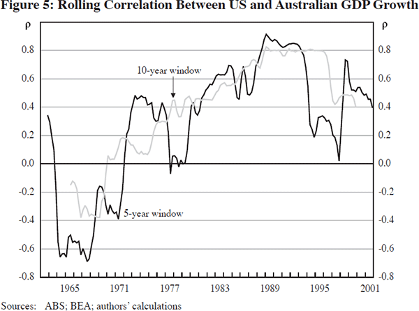
Table 7 presents dynamic correlations between leads and lags of US and Australian growth rates over the whole sample and across the main sub-samples of Table 3. The dynamic correlations suggest a substantially stronger correlation between lags of US GDP and Australian GDP than the reverse, consistent with the US economy leading the Australian economy – once again it is clear that this relationship has strengthened significantly since the mid 1970s.
| Correlations | 1960:Q1–2004:Q4 | 1960:Q1–1982:Q4 | 1983:Q1–2004:Q4 | 1960:Q1–1973:Q4 | 1974:Q1–2004:Q4 |
|---|---|---|---|---|---|
| ρ(Aust, USt−4) | 0.32 | 0.19 | 0.47 | 0.27 | 0.26 |
| ρ(Aust, USt−3) | 0.44 | 0.30 | 0.56 | 0.22 | 0.46 |
| ρ(Aust, USt−2) | 0.47 | 0.28 | 0.64 | 0.10 | 0.54 |
| ρ(Aust, USt−1) | 0.43 | 0.19 | 0.65 | −0.17 | 0.57 |
| ρ(Aust, USt) | 0.33 | 0.23 | 0.59 | −0.15 | 0.53 |
| ρ(Aust, USt+1) | 0.22 | 0.01 | 0.44 | −0.40 | 0.35 |
| ρ(Aust, USt+2) | 0.09 | −0.04 | 0.23 | −0.32 | 0.14 |
| ρ(Aust, USt+3) | 0.01 | 0.01 | 0.04 | −0.11 | −0.05 |
| ρ(Aust, USt+4) | −0.06 | 0.00 | −0.08 | 0.02 | −0.23 |
|
Sources: authors' calculations, using ABS and BEA |
|||||
4.3 Allowing for time-varying GDP growth and volatility
One possible explanation for the increase in the correlation between Australian and US GDP is that structural breaks in the mean or variance of GDP growth in one or both countries have affected the correlation over certain sub-samples. In both countries a decline in the volatility of GDP growth has been documented, and there is also some evidence of a fall in the mean GDP growth rate, at least in the case of Australia.
Many papers have documented the decline in volatility in the US economy starting in the mid 1980s, although there has been some debate over whether the decline has been smooth or due to a one-off shift, as well as potential causes of the decline (see Blanchard and Simon 2001, and McConnell and Perez-Quiros 2000). These papers find no apparent break in the mean growth rate of GDP (no shift in potential GDP) for the US, despite the much discussed productivity slowdown in the 1980s and the ‘IT revolution’ beginning in the mid to late 1990s.
In Australia, however, there is evidence of a break in mean GDP growth in the early 1970s as well as a similar decline in volatility to the US in the mid 1980s. The permanent fall in average GDP growth in the early 1970s in Australia, from around 5 per cent per annum to just over 3 per cent per annum, is fairly similar in timing and magnitude to the fall experienced in Canada (see Debs 2001 and Voss 2004), although Canada seems to have experienced increasing volatility in GDP growth in the 1980s and 1990s – the opposite of the Australian and US experience. Figure 6 illustrates the permanent slowdown in Australian growth around the time of the first oil shock.
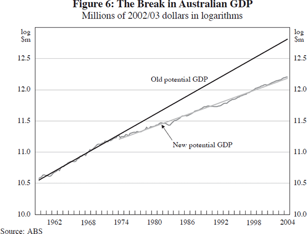
The Australian data do not show any evidence of a pick-up in productivity and GDP growth since the mid 1990s. Whilst trend growth has increased in Australia after 1995, from around 3 per cent per annum to over 4 per cent per annum (still well below the 5 per cent-plus average growth rates of the 1960s), this spurt in economic growth was not sustained into the new millenium. Average growth rates since 2000 have been, at best, similar to those experienced since 1971.
More formal evidence regarding the instability in the conditional moments of Australian and US GDP is provided in Table 8. Following Stock and Watson (2002), we conduct Andrews-Quandt-type break tests on the coefficients of an autoregressive model that allows either the conditional mean or the conditional variance, or both, to break, possibly at different dates. The estimated model is of the form,

where

ø1(L) and ø2(L) are lag polynomials, and κ and τ are the break dates for the conditional mean and conditional variance respectively. The sup-Wald statistics (see Andrews 1993) used to test the stability of the conditional mean are computed for all possible break dates in the central 70 per cent of the sample. To test the stability of the conditional variance, the growth rate series was first demeaned, allowing for any break in mean found for the series, and the sup-Wald test statistics calculated for the residuals from the estimated regression run on the demeaned data.
| Real GDP growth | Sup-Wald test | p-value | Break date |
|---|---|---|---|
| US conditional mean | 10.79 | 0.47 | – |
| Australian conditional mean | 26.88 | 0.00 | 1971:Q3 |
| US conditional standard deviation (constant mean) |
27.60 | 0.00 | 1984:Q4 |
| Australian conditional standard deviation (break in mean: 1971:Q3) |
34.88 | 0.00 | 1982:Q1 |
| Correlation of demeaned growth rates | 27.01 | 0.00 | 1973:Q4 |
| Note: Bold type indicates significance at the 5 per cent level. | |||
Table 8 suggests that there is no significant break in the conditional mean of the US GDP growth series but there is strong evidence of a structural break in 1971:Q3 for Australia, somewhat before the occurrence of the first oil price shock. Filtering the GDP growth rates on the basis of these results gave the demeaned growth rates as depicted in Figure 7.
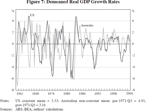
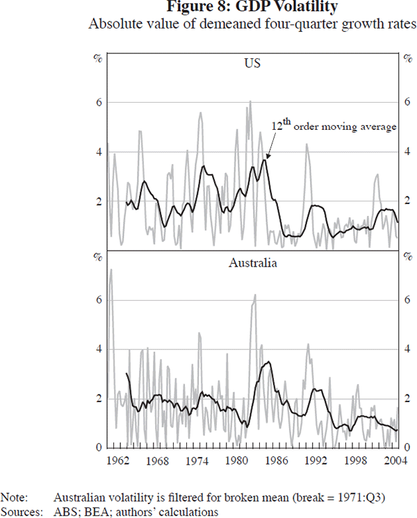
Using these demeaned growth rates in the time-varying autoregressive models, tests were then performed on the stability of the conditional variances. The sup-Wald test statistics provide strong evidence of significant breaks in volatility for both economies. The evidence suggests a break in the US series towards the end of 1984, consistent with the date suggested by McConnell and Perez-Quiros (2000), Stock and Watson (2002) and Voss (2004).[3] The sup-Wald test statistic suggests that the break date for Australia is 1982:Q1. Time-varying measures of volatility – the absolute value of the demeaned four-quarter growth rates for each country and a simple 12th order moving average – are depicted in Figure 8. This provides further visual evidence of the decline in volatility in both countries.
Finally, to test the stability of the correlation between US and Australian growth rates, the sup-Wald test statistic was calculated for the coefficient on the US GDP growth rate in a simple regression of the demeaned Australian growth rate on the US growth rate. The test provides strong evidence of a significant shift in the correlation between Australian and US growth rates in 1973:Q4 after the recession caused by the first oil shock, thus formalising the break date suggested by the correlations in Table 6 and by Figure 5.
5. Understanding the Changing Correlation
In the previous section we provided evidence that both the US and Australian economies have undergone shifts in either mean growth rates, volatility, or both, and that the two economies moved towards a much higher degree of correlation with each other after the recession of the early 1970s. We now present some evidence as to why the Australian economy might have moved so much closer in terms of its cyclical variation to that of the US. In turn this will allow us to ask whether such changes are likely to persist into the future. We begin by examining the components of Australian GDP. This allows us to answer questions such as whether Australia's exports respond to US GDP growth in the same manner as Australia's GDP. We then examine some other macroeconomic variables, such as interest rates and employment growth. To fully understand changes in the correlation patterns a more structural approach would be preferable, but we think that the findings in this section are useful pointers for further research.
5.1 Correlations with Australian GDP components
Tables 9 and 10 present detail on the components of Australian GDP along similar lines to the evidence on GDP in Section 4. Table 9 shows that the mean and variance profiles of the Australian components are similar to the equivalent US components. The correlations with US components and with US GDP suggest that investment is the component of Australia's GDP that most closely tracks US GDP. In the 1970s and 1990s, Australian investment was highly correlated with US investment and US GDP. Interestingly the correlation dropped away in the 1980s. However, the overall pattern in Table 9 is suggestive that supply or productivity shocks in the 1990s were similar in Australia and the US, driving the high correlation between Australian and US investment and GDP.
| 1961–2004 | 1960s | 1970s | 1980s | 1990s | 2000s | 1961–1982 | 1983–2004 | |
|---|---|---|---|---|---|---|---|---|
| Mean | ||||||||
| GDP | 3.59 | 4.84 | 3.33 | 3.28 | 3.24 | 3.19 | 3.79 | 3.39 |
| Consumption | 3.55 | 4.51 | 3.55 | 3.10 | 3.19 | 3.36 | 3.95 | 3.11 |
| Investment | 3.96 | 5.27 | 2.26 | 4.69 | 3.46 | 4.81 | 3.90 | 4.02 |
| Δ inventories/GDP | 0.31 | – | 0.64 | 0.33 | 0.16 | 0.13 | 0.53 | 0.21 |
| Exports | 5.87 | 7.30 | 5.47 | 4.69 | 7.16 | 3.03 | 5.63 | 6.13 |
| Imports | 5.45 | 5.72 | 3.65 | 6.61 | 5.78 | 5.63 | 4.88 | 6.06 |
| Standard deviation | ||||||||
| GDP | 2.35 | 2.87 | 2.28 | 2.56 | 1.83 | 1.05 | 2.68 | 1.96 |
| Consumption | 1.74 | 2.14 | 1.68 | 1.55 | 1.55 | 0.67 | 1.87 | 1.48 |
| Investment | 6.25 | 3.14 | 4.33 | 7.42 | 7.26 | 9.19 | 4.52 | 7.71 |
| Δ inventories/GDP | 0.82 | – | 1.01 | 0.84 | 0.76 | 0.34 | 0.91 | 0.76 |
| Exports | 7.03 | 9.16 | 6.67 | 7.65 | 4.11 | 5.69 | 7.98 | 5.88 |
| Imports | 10.50 | 12.12 | 12.69 | 10.94 | 6.33 | 7.73 | 11.80 | 8.92 |
| Standard deviation relative to US equivalent component | ||||||||
| Consumption | 0.94 | 1.33 | 0.76 | 0.78 | 1.07 | 0.76 | 0.84 | 0.94 |
| Investment | 1.10 | 0.89 | 0.61 | 1.13 | 1.54 | 2.34 | 0.74 | 1.10 |
| Δ inventories/GDP | 1.54 | – | 2.05 | 1.40 | 1.96 | 0.58 | 1.53 | 1.50 |
| Exports | 1.08 | 1.54 | 0.92 | 1.06 | 1.14 | 0.74 | 1.12 | 1.08 |
| Imports | 1.45 | 1.96 | 1.42 | 1.31 | 1.48 | 1.05 | 1.46 | 1.45 |
| Correlation with US equivalent component | ||||||||
| GDP | 0.34 | −0.05 | 0.08 | 0.57 | 0.80 | 0.28 | 0.24 | 0.59 |
| Consumption | 0.17 | 0.24 | −0.06 | −0.34 | 0.73 | 0.33 | 0.15 | 0.22 |
| Investment | 0.36 | 0.35 | 0.51 | 0.19 | 0.87 | −0.20 | 0.33 | 0.41 |
| Δ inventories/GDP | 0.30 | – | 0.11 | 0.47 | 0.24 | 0.07 | 0.23 | 0.35 |
| Exports | 0.05 | −0.22 | −0.29 | 0.21 | 0.46 | 0.80 | −0.22 | 0.54 |
| Imports | 0.21 | −0.06 | 0.27 | 0.11 | 0.81 | 0.55 | 0.12 | 0.37 |
| Correlation with US GDP growth | ||||||||
| Consumption | 0.16 | 0.14 | −0.07 | −0.16 | 0.70 | 0.33 | 0.14 | 0.21 |
| Investment | 0.37 | 0.35 | 0.54 | 0.21 | 0.86 | 0.03 | 0.39 | 0.48 |
| Exports | −0.04 | −0.40 | −0.26 | 0.28 | −0.37 | 0.74 | −0.14 | 0.16 |
| Imports | 0.13 | −0.12 | 0.05 | 0.20 | 0.76 | 0.59 | −0.02 | 0.50 |
|
Note: The change in inventories is measured in similar fashion to Stock and Watson (2002) as 100 x (Δ inventories/GDP) and is over the sample of 1974:Q3–2003:Q4 only. Sources: authors' calculations, using ABS and BEA |
||||||||
| Australian GDP component | Sup-Wald test | p-value | Likely break date |
|---|---|---|---|
| Conditional mean | |||
| Output (GDPt) | 26.88 | 0.00 | 1971:Q3 |
| Consumption (Ct) | 23.16 | 0.01 | 1978:Q2 |
| Investment (It) | 13.02 | 0.26 | 1967:Q4 |
| Δ inventories/GDP | 8.85 | 0.68 | 1979:Q3 |
| Exports (Expt) | 3.57 | 0.45 | 1969:Q3 |
| Imports (Impt) | 17.29 | 0.07 | 1979:Q1 |
| Unconditional standard deviation | |||
| Output (GDPt) | 17.33 | 0.00 | 1992:Q2 |
| Consumption (Ct) | 11.27 | 0.02 | 1991:Q4 |
| Investment (It) | 28.54 | 0.00 | 1980:Q2 |
| Δ inventories/GDP | 7.32 | 0.09 | 1979:Q3 |
| Exports (Expt) | 18.66 | 0.00 | 1967:Q2 |
| Imports (Impt) | 20.55 | 0.00 | 1991:Q3 |
| Conditional standard deviation | |||
| Output (GDPt) | 34.88 | 0.00 | 1982:Q1 |
| Consumption (Ct) | 7.64 | 0.81 | 1994:Q3 |
| Investment (It) | 13.11 | 0.25 | 1982:Q2 |
| Δ inventories/GDP | 9.17 | 0.64 | 1979:Q3 |
| Exports (Expt) | 7.53 | 0.82 | 1973:Q4 |
| Imports (Impt) | 9.05 | 0.65 | 1991:Q1 |
| Correlation with US equivalent | |||
| ρ(AusCt, USCt) | 14.68 | 0.00 | 1990:Q2 |
| ρ(AusIt, USIt) | 9.39 | 0.04 | 1984:Q4 |
| ρ(AusInventoriest, USInventoriest) | 4.10 | 0.36 | 1993:Q3 |
| ρ(AusExpt, USExpt) | 24.68 | 0.00 | 1982:Q4 |
| ρ(AusImpt, USImpt) | 11.42 | 0.01 | 1974:Q4 |
| Correlation with demeaned US GDP | |||
| ρ(AusCt, USGDPt) | 12.64 | 0.01 | 1985:Q2 |
| ρ(AusIt, USGDPt) | 21.02 | 0.00 | 1984:Q4 |
| ρ(AusExpt, USGDPt) | 5.78 | 0.18 | 1979:Q4 |
| ρ(AusImpt, USGDPt) | 16.20 | 0.00 | 1974:Q4 |
|
Note: Bold type indicates significance at the 10 per cent level. Source: authors' calculations |
|||
Table 10 tests for constancy of the means and variances of the GDP components, as well as the stability of correlations. When considering the different components it appears from the break dates that the correlations rise at a later date than those of GDP itself.
5.2 Monetary policy
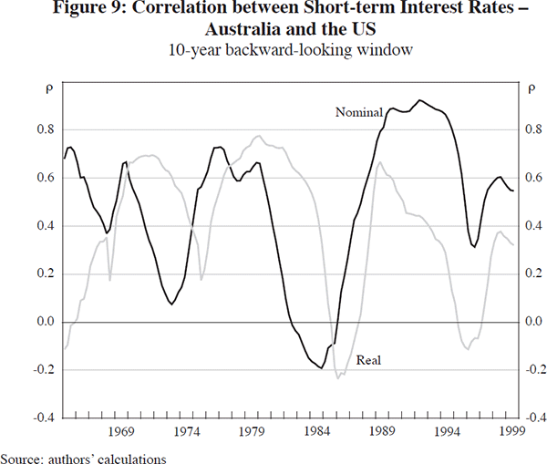
Table 11 details the behaviour of some other Australian macroeconomic variables. Nominal interest rates are highly correlated with US interest rates, except in the 1980s, while real interest rates show a pattern similar to GDP correlations – real rates were negatively correlated in the 1960s, but the correlation then increases in the 1970s and 1980s. However, the correlation between real rates is not evident beyond 1990. Interestingly, the graph of rolling 10-year correlations shown in Figure 9 clearly illustrates the similarity of monetary policy during the 1980 and 1990 recessions. In both countries these recessions were periods of very tight monetary policy as inflation was brought under control. It may be that the structural break tests (Table 12) and the correlation patterns decade by decade are not picking up similarity in monetary policy that was specific to a very small number of years over the sample.
| Full sample | 1960s | 1970s | 1980s | 1990s | 2000s | |
|---|---|---|---|---|---|---|
| Mean | ||||||
| Cash rate | 6.18 | 3.85 | 6.85 | 14.03 | 7.24 | 5.11 |
| Cash rate (real) | 2.13 | 1.35 | −3.16 | 5.66 | 4.88 | 1.68 |
| M3 growth | 10.74 | – | 11.82 | 13.17 | 8.12 | 8.93 |
| Inflation | 5.31 | 2.44 | 9.29 | 8.06 | 2.46 | 3.33 |
| Δ inflation | 0.00 | 0.00 | 0.17 | −0.05 | −0.14 | 0.02 |
| Employment | 2.05 | 2.89 | 1.63 | 2.40 | 1.23 | 2.18 |
| Standard deviation | ||||||
| Cash rate | 4.20 | 0.70 | 2.92 | 2.99 | 1.01 | 0.42 |
| Cash rate (real) | 4.14 | 1.36 | 4.41 | 2.30 | 1.71 | 1.23 |
| M3 growth | 4.41 | – | 5.24 | 3.97 | 2.84 | 2.17 |
| Inflation | 3.87 | 1.51 | 3.77 | 2.08 | 2.07 | 1.32 |
| Δ inflation | 0.99 | 0.82 | 1.26 | 1.02 | 0.76 | 1.10 |
| Employment | 1.68 | 1.10 | 5.75 | 2.04 | 1.86 | 0.90 |
| Correlation with US equivalent | ||||||
| Cash rate | 0.64 | 0.66 | 0.41 | −0.15 | 0.77 | 0.74 |
| Cash rate (real) | 0.59 | −0.11 | 0.36 | 0.23 | 0.08 | −0.72 |
| M3 growth | 0.14 | – | −0.09 | −0.74 | 0.16 | 0.20 |
| Inflation | 0.71 | 0.29 | 0.57 | 0.33 | 0.76 | 0.58 |
| Δ inflation | 0.13 | −0.23 | 0.30 | −0.10 | 0.30 | 0.45 |
| Employment | 0.43 | 0.57 | 0.06 | 0.61 | 0.81 | 0.23 |
|
Notes: Variables are levels of 10-year, 90-day interest rates and annualised inflation rates, period-by-period change in annualised inflation, and four-quarter growth rates of seasonally adjusted M3 and non-farm employment. Sources: authors' calculations, using ABS and RBA |
||||||
| Australian variable | Sup-Wald test | p-value | Likely break date |
|---|---|---|---|
| Conditional mean | |||
| Cash rate | 22.37 | 0.01 | 1986:Q3 |
| Cash rate (real) | 14.02 | 0.19 | 1976:Q4 |
| M3 growth rate (M3t) | 18.82 | 0.04 | 1990:Q4 |
| Inflation (πt) | 12.02 | 0.33 | 1990:Q4 |
| Δ inflation (Δπt) | 7.28 | 0.85 | 1975:Q1 |
| Employment growth (Empt) | 8.48 | 0.72 | 1997:Q3 |
| Unconditional standard deviation | |||
| Cash rate | 24.06 | 0.00 | 1991:Q2 |
| Cash rate (real) | 23.57 | 0.00 | 1992:Q3 |
| M3 growth rate (M3t) | 30.13 | 0.00 | 1976:Q1 |
| Inflation (πt) | 12.55 | 0.01 | 1983:Q3 |
| Δ inflation (Δπt) | 4.05 | 0.37 | 1985:Q3 |
| Employment growth (Empt) | 17.93 | 0.00 | 1995:Q4 |
| Conditional standard deviation | |||
| Cash rate | 24.67 | 0.00 | 1983:Q1 |
| Cash rate (real) | 10.17 | 0.52 | 1974:Q4 |
| M3 growth rate (M3t) | 25.58 | 0.00 | 1975:Q3 |
| Inflation (πt) | 11.37 | 0.40 | 1975:Q2 |
| Δ inflation (Δπt) | 8.55 | 0.71 | 1991:Q4 |
| Employment growth (Empt) | 12.54 | 0.29 | 1997:Q3 |
| Correlation with US equivalent | |||
| ρ(casht, fedfundst) | 82.24 | 0.00 | 1982:Q1 |
| ρ(realcasht, realfundst) | 28.71 | 0.00 | 1983:Q4 |
| ρ(AusM3t, USM3t) | 9.60 | 0.11 | 1990:Q2 |
| ρ(Ausπt, USπt) | 19.44 | 0.00 | 1991:Q3 |
| ρ(AusΔπt, USΔπt) | 6.06 | 0.16 | 1990:Q3 |
| ρ(AusEmpt, USEmpt) | 19.45 | 0.00 | 1982:Q2 |
|
Note: Bold type indicates significance at the 5 per cent level. Source: authors' calculations |
|||
5.3 Looking ahead – will a growing China affect Australia?
Thus far in this section we have suggested that the Australian economy has been synchronised with the US and other economies in the post-war period mainly through synchronisation of monetary policy in the early 1980s and early 1990s, and the oil shock that affected global economies in the early 1970s. Currently, however, there is a debate in Australia about how closely the Australian economy is tied to the growth of the Chinese economy. One suggestion is that with the Australian resources sector and terms of trade heavily affected by China's growth, a slowdown in China will have serious negative consequences for the Australian economy.
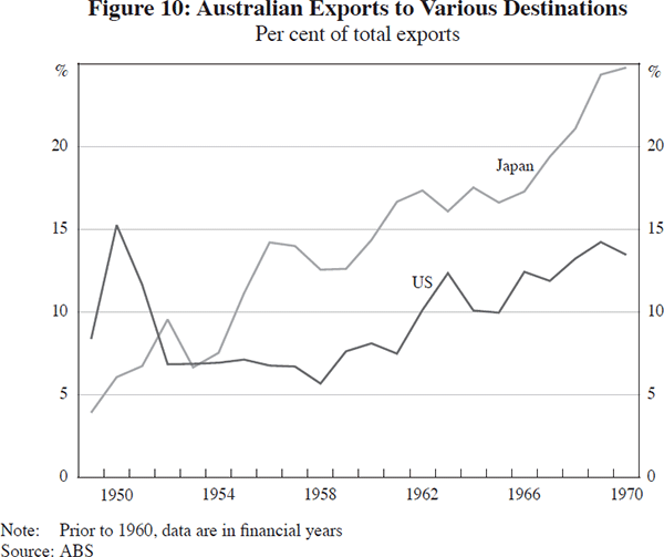
We do not see risks associated with Australia's stronger trade relationships with China for two reasons. First, as discussed in Crosby (2004), we see it as unlikely that China's medium- to longer-term outlook will deteriorate, so that trade between Australia and China will continue to grow steadily. Second, we do not expect that any hiccup to China's growth will cause recession in Australia. In Figure 10 we show Japan's share of Australian trade from 1949 to 1970. During this period Japan's share of Australia's exports rose from around 4 per cent to almost 25 per cent. Despite this rise, the correlation between Australian and Japanese GDP growth in the 1960s is zero, as shown in Table 3. Japan remains Australia's major trading partner, but the poor performance of the Japanese economy since 1990 has not stopped Australia from achieving strong rates of economic growth since this time.
6. Conclusions
In this paper we examine the issue of whether or not the Australian economy is inexorably linked to the US economy. We argue that the pattern of a strong post-war correlation between Australian and US GDP is largely explained through the experience of three deep recessions with very similar timing. The latter two recessions were associated with very high real interest rates in both countries, and are commonly described as recessions in which monetary policy played a very prominent role. This high level of policy synchronisation can explain why the Australian economy has become more synchronised with the US since 1980, a pattern which is the opposite of that for other OECD economies studied in Heathcote and Perri (2003).
Prior to World War II the Australian and the US economies were not at all synchronised, despite economic structures that appeared quite similar. The only years during this period when the two economies were synchronised were during the 1890s recession and during the Depression years. Looking ahead, with both countries likely to achieve low inflation into the foreseeable future, one cannot see a high probability of monetary policy-induced recessions that occurred in the 1980s and 1990s. If the global economy catches a cold then Australia will no doubt be affected, but Australia has less to fear from idiosyncratic recessions in any particular major economy.
Footnotes
Using a Google search we were able to find 110 such quotes in the press or on radio transcripts in Australia over the last 5 years. [1]
The correlation patterns between lags of Australian GDP and the other countries' GDP are similar. [2]
Voss suggests a break date for volatility for the US of 1985:Q1 whilst Stock and Watson provide a confidence interval for their US break date of 1982:Q4–1985:Q3. [3]
References
Andrews DWK (1993), ‘Tests for parameter instability and structural change with unknown change point’, Econometrica, 61(4), pp 821–856.
Bambrick S (1970), ‘Australia's long run terms of trade’, Economic Development and Cultural Change, 19(1), pp 1–5.
Blanchard OJ and J Simon (2001), ‘The long and large decline in U.S. output volatility’, Brookings Papers on Economic Activity, 1, pp 135–164.
Butlin NG (1962), Australian domestic product, investment and foreign borrowing 1861–1938/39, Cambridge University Press, Cambridge.
Butlin NG (1985), ‘Australian national accounts 1788–1983’, ANU Source Papers in Economic History No 6.
Clark TE and E van Wincoop (2001), ‘Borders and business cycles’, Journal of International Economics, 55(1), pp 59–85.
Crosby M (2003), ‘Business cycle correlations in Asia-Pacific’, Economic Letters, 80(1), pp 35–44.
Crosby M (2004), ‘Chinese economic growth and the Australian economy’, Mercer-Melbourne Institute Quarterly Bulletin of Economic Trends, 4.04, pp 21–22.
Debs A (2001), ‘Testing for a structural break in the volatility of real GDP growth in Canada’, Bank of Canada Working Paper No 2001-9.
Frankel JA and AK Rose (1998), ‘The endogeneity of the optimum currency area criteria’, Economic Journal, 108(449), pp 1009–1025.
Heathcote J and F Perri (2003), ‘Why has the US economy become less correlated with the rest of the world?’, American Economic Review, Papers and Proceedings, 93(2), pp 63–69.
Imbs J (2000), ‘Sectors and the OECD business cycle’, Centre for Economic Policy Research Discussion Paper Series No 2473.
Imbs J (2004), ‘Trade, finance, specialization, and synchronization’, Review of Economics and Statistics, 86(3), pp 723–734.
Kose MA, ES Prasad and ME Terrones (2003), ‘How does globalization affect the synchronization of business cycles?’, American Economic Review, Papers and Proceedings, 93(2), pp 57–62.
Lee SP and P Passell (1979), A new economic view of American history, WW Norton & Company, New York.
Maddison A (1995), Monitoring the world economy, 1820–1992, OECD Development Centre, Washington DC.
McConnell MM and G Perez-Quiros (2000), ‘Output fluctuations in the United States: what has changed since the early 1980s?’, American Economic Review, 90(5), pp 1464–1476.
Meredith D and B Dyster (1999), Australia in the global economy, Cambridge University Press, Port Melbourne.
Mitchell BR (1988), British historical statistics, Cambridge University Press, Cambridge.
Otto G, G Voss and L Willard (2001), ‘Understanding OECD output correlations’, Reserve Bank of Australia Research Discussion Paper No 2001-05.
Pagan A (1996), ‘The rise and fall and rise … of the business cycle’, Australian National University Centre for Economic Policy Research Discussion Paper No 349.
Rose AK and C Engel (2000), ‘Currency unions and international integration’, NBER Working Paper No 7872.
Stock JH and MW Watson (2002), ‘Has the business cycle changed and why?’, in M Gertler and K Rogoff (eds), NBER macroeconomics annual 2002, MIT Press, Cambridge, pp 159–218.
United States Bureau of the Census (1975), Historical statistics of the United States, colonial times to 1970, Government Printing Office, Washington DC.
Voss GM (2004), ‘Aspects of Canadian and US business cycles’, University of Victoria manuscript.
Williamson JG (1964), American growth and the balance of payments, 1820–1913, University of North Carolina Press, Chapel Hill.