RBA Annual Conference – 2005 Financial System Liquidity, Asset Prices and Monetary Policy Hyun Song Shin^[1]

1. Introduction

Monetary policy works by manipulating asset prices, especially long-term interest rates. Although a central bank generally directly controls only the overnight interest rate, its communication policy serves to guide the market's expectations into doing its bidding. By moulding market expectations, the central bank can manipulate long-term interest rates, and thereby affect mortgage rates, corporate lending rates and other prices that have a direct impact on the economy.

However, even though financial markets are the medium through which the central bank gives effect to its monetary policy, the consequences of the central bank's actions are seen almost exclusively through the lens of the IS curve – that is, through quantities such as consumption and investment. The wider consequences of monetary policy for the financial system as a whole receive less weight in central bank pronouncements on monetary policy. The task of maintaining financial stability is allocated to the central bank's role (if any) in financial supervision and prudential regulation. In effect, a Tinbergen-style allocation of instruments to goals is envisaged where the goal of monetary policy is to ensure price stability, and supervisory/prudential policy is aimed at financial stability. This allocation of roles is neatly summarised in a speech by Fed Governor Ben Bernanke (2002):

… as a general rule, the Fed will do best by focusing its monetary policy instruments on achieving its macro goals – price stability and maximum sustainable employment – while using its regulatory, supervisory, and lender-of-last resort powers to help ensure financial stability.

It is not my intention here to revisit the debate on whether it is better for the central bank to attempt to ‘prick’ a suspected asset-price bubble or whether instead it should wait for the bubble to burst of its own accord, and work toward softening the impact of the resulting downturn.^[2] In one sense, this debate is not entirely helpful since it takes for granted the existence (or suspected existence) of an asset-price bubble, and the focus is on how to deal with it once it has taken hold. What is less widely discussed is how monetary policy may contribute to the inflating of an asset-price bubble in the first place. It is this issue that I attempt to address in what follows.

The role of monetary policy in setting the general tenor of financial market conditions has returned as a topical issue in the wake of the unprecedented monetary easing in the US in recent years. Commentators are fond of using expressions such as the financial markets being ‘awash with liquidity’, leading to compressed yield spreads and the chasing of yields. Indeed, recent developments in financial markets have posed a challenge to central bankers and other public officials. Signals emanating from the financial markets – in the form of low long-term interest rates, compressed yield spreads and low implied volatility – seem to paint an implausibly benign economic picture that gives very little weight to the potential sources of downside risk.^[3]

More recently, the debate in the US (on the heels of similar debates in Australia and many other countries) has moved to the relationship between monetary policy and its role in fuelling the rise in the price of residential property. Fed Governor Donald Kohn (2005) puts the matter thus:

Low interest rates have, in turn, been a major force driving the phenomenal run-up in residential real estate prices over the past few years, and the resultant boost to net worth must be one of the reasons households have felt comfortable directing so little of their current income to saving. However, whether low interest rates and other fundamental factors can fully explain the current lofty level of housing prices is the subject of substantial debate.

The purpose of my paper is to shed some additional light on this debate. To the extent that monetary policy works by manipulating asset prices – in particular, long-term interest rates – we may expect broader repercussions on financial institutions and markets through changes in the relative values of liabilities and assets (and hence net worth), the availability of credit, and asset prices. Inevitably, such effects will harbour feedback elements that serve to magnify the responses to initial shocks. Balance-sheet changes will affect asset prices and asset-price changes will affect balance sheets. The loop thus created will generate amplified responses to the changing of monetary policy.

The literature on the transmission of monetary policy has distinguished two potential ‘credit channels’ through which monetary policy affects lending. The first is the increased credit that operates through the borrowers' balance sheets, where increased lending comes from the greater creditworthiness of the borrower (Bernanke and Gertler 1989; Kiyotaki and Moore 1998, 2001a, 2001b). The second is the channel that operates through the banks' balance sheets (the ‘bank lending channel’), where open market operations that drain reserves would limit bank loans by reducing banks' access to loanable funds (Bernanke and Blinder 1988; Kashyap and Stein 2000).

The channel explored in my paper is a variation of the second, and emphasises the net worth of the banks themselves, and the incentive effects to restore leverage when balance sheets are continuously marked to market. Van den Heuvel's (2002a, 2002b) notion of the ‘bank capital channel’ is most closely related to the ideas explored here. Although the assumption of continuous marking to market is not appropriate if taken literally, the ‘banks’ in my framework could be seen as the US mortgage agencies such as Fannie Mae, that deal mainly with marketable claims. In any case, I will argue below that trends in financial markets and accounting rules are likely to make marking to market more important in determining the behaviour of financial institutions.

The amplified response to the easing of monetary policy, by itself, need not be a problem for policy-makers if they can fine-tune their monetary policy levers to take account of the amplification. Rather, the problem is the highly asymmetric nature of the mechanisms at play ‘on the way up’ versus the mechanisms ‘on the way down’. If the bursting of a property bubble impairs the solvency of the financial sector, then the dynamics ‘on the way down’ can turn into an extremely messy affair, involving a whole new set of mechanisms that did not figure in the initial inflating of the bubble. Default, financial distress, and inefficient liquidations will all conspire to exact very large economic costs.

Marked-to-market snapshots of the household balance sheet cannot always be relied on as a source of comfort. Although the marked-to-market value of the residential housing stock goes up in proportion to the current market price (assuming a fixed housing stock), this increase in the value of the housing stock cannot be seen as an increase in net wealth for the economy as a whole. It merely reflects the reallocation of housing between households – or more accurately, the rate at which the marginal reallocation takes place. The shift is within the Edgeworth box, rather than an expansion of the Edgeworth box.

The new holders of the housing stock may (almost tautologically) have a higher consumption value for housing, but this higher consumption value is not fungible, and so is not available for repayment of debt. It is only when the indebted households can rely on a secure, independent stream of cash flow (say, from wage income) that debt service is assured. It is one of the tenets of good banking practice that the banker should look at the borrower's future cash flows, rather than be fixated by the value of the borrower's collateral assets. Japanese banks were reminded of the wisdom of this rule following the bursting of the property bubble there.

Marking the current housing stock to market can create a misleading impression of the strength of aggregate balance sheets. Consider the following passage from a recent commentary in the Wall Street Journal:^[4]

While many believe that irresponsible borrowing is creating a bubble in housing, this is not necessarily true. At the end of 2004, U.S. households owned $17.2 trillion in housing assets, an increase of 18.1% (or $2.6 trillion) from the third quarter of 2003. Over the same five quarters, mortgage debt (including home equity lines) rose $1.1 trillion to $7.5 trillion. The result: a $1.5 trillion increase in net housing equity over the past 15 months.

The author minimises the dangers from the $1.1 trillion increase in indebtedness by appealing to the marked-to-market value of housing equity. The counterargument would be that the marked-to-market value of the housing stock (assessed at the current marginal transaction price) may not be a good indicator of the strength of the aggregate household sector balance sheet. In aggregate terms, the relevant question is how much value can be realised if a substantial proportion of the housing stock were to be put up for sale. The value realised in such a sale would be much smaller than the current marked-to-market value. This is one instance in which marking to market gives a misleading indicator of the aggregate position.^[5]

It is not inevitable that the bursting of a property bubble undermines the financial system as a whole. The experience in Hong Kong following the bursting of the housing bubble in 1997 is a case in point. Residential property prices declined by around 70 per cent in Hong Kong between 1997 and 2004, but there was no banking crisis. There are important lessons to be learned from the Hong Kong experience. Loan-to-value ratios were generally very low in Hong Kong. Also, households continued to service their debt, even though the value of their houses fell far short of their mortgage obligations, pointing to the importance of the bankruptcy regime in place. If the borrower can declare bankruptcy, return the keys, and walk away, then it is the banking sector that will end up holding the depreciating property stock. It is unclear how far Hong Kong's experience can be extrapolated to the US, Australia, Spain and the many other countries that have experienced residential property booms. Loan-to-value ratios and bankruptcy rules may differ substantially from those in place in Hong Kong.

More systematic empirical evidence is not so encouraging for a country that undergoes a property-price boom financed by large increases in private credit. Borio and Lowe (2002a, 2002b, 2004) exhibit evidence that the joint occurrence of property booms and ‘excessive’ private-sector credit growth help predict banking distress, economic weakness and disinflation over a three- to five-year horizon. The important point is that even as financial imbalances build up, goods price inflation can remain low and stable (Japan in the 1980s being a prime example).

I begin the main body of the paper by outlining a general framework for examining the interrelationships between the value of obligations in a system of interlocking balance sheets, which is then applied to a highly stylised model of an economy with property as the sole real asset. The amplifying effect of monetary easing and its effect in raising property prices is illustrated within the stylised model. In keeping with the theme of this year's RBA conference – on the changing nature of the business cycle – I close by outlining a number of factors affecting financial institutions and markets that have served to sharpen the effects outlined here.

2. Framework for a Financial System

The basic problem can be posed in the following way. The marked-to-market value of my claim against A depends on A's creditworthiness, and so depends on the value of A's claims against B, C, etc. However, B or C may have a claim against me, and so we are back full circle. The task of valuing claims in a financial system thus entails solving for a consistent set of prices – that is, solving a fixed-point problem.

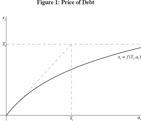
Suppose that borrower i has issued debt with face value , and has assets with market value a_i. The market value of i's debt, denoted by x_i, is less than its face value, but is increasing in the value of i's assets. Denote by f_i(,a_i) the market value of i's debt with face value when i's assets have market value a_i. Figure 1 depicts this relationship. As noted by Merton (1974), the market value of i's debt is the price of a short position in a put option on i's assets with strike price equal to the face value of the debt. Among other things, this implies that x_i is increasing in , and is also increasing in a_i, but the slope is less than 1 everywhere.

The value of i's assets will depend, in part, on the value of his claims against other borrowers in the financial system. The value of i's assets will also depend on the prices of real assets (assets that are not the obligations of some other party). Suppose that there is only one type of real asset in the economy, and denote its price by v. We thus have the following system for the determination of the value of financial system claims:

The notation a_i(x,v) reflects the fact that the value of i's assets depends on the vector of all claims in the financial system (given by x) as well as the price of the real asset. More succinctly, we can write this system as

A consistent set of valuations is a fixed point x of the mapping F. The following set of results can be shown ^[6] to hold in this setting:

• there is a unique fixed point x of the mapping F;
• x is increasing in ; and
• x can be computed numerically as the limit of the sequence F(0), F²(0), F³(0), … where Fⁿ(0) is the n-fold composition of the mapping F on the zero vector.

If the level of debt (as given by the vector ) is endogenously chosen by the constituents of the system themselves, then there is the potential for feedback from (the level of indebtedness) to v (the price of the real asset) to x (the market value of claims/obligations). Since x determines the net worth of the financial system constituents, this in turn influences the decisions on . We would then be back full circle, and another round of increases (decreases) will take place. When the sole real asset is property, the feedback can be described in terms of a property boom (bust) being fuelled by the buoyancy (weakness) of demand as reflected in the availability of credit and the health of balance sheets.

Assessing financial claims in a system setting captures a number of features that are missing in a partial equilibrium setting. For instance, it is possible for spreads to fall as debts rise. If v is sufficiently sensitive to the flow of new funds into the property sector, then the increase in market values x can be so large as to swamp the increase in face values . Symmetrically, it is possible that de-leveraging leads to increases in spreads (as is often observed during crises).

In any case, property prices, creditworthiness and the level of debt are all interrelated, and we could call the snapshot of the current state of these variables the state of ‘financial system liquidity’. Into this heady mix comes monetary policy. Monetary policy operates by manipulating the prices of treasury securities – in particular by manipulating (through the central bank's policy rate and its communication policy) the prices of long-dated treasuries. When monetary policy is loosened, for example, long-duration assets (and liabilities) will gain in value by more than short-duration assets/liabilities. Thus, the market value of claims and obligations (given by the vector x) will shift, affecting the balance sheets of the financial system constituents. When x shifts, so will and hence v. In this way, an easing of monetary policy can be expected to have an impact on the overall level of debt through changes in net worth and the creditworthiness of borrowers. The overall level of debt then has an impact on the real asset price. In concrete terms, banks that borrow short and lend long will experience an increase in their market net worth, and may react to their stronger balance-sheet position by increasing their lending. Increased credit will lead to a rise in the real asset price.

Having outlined the basic framework in general terms, I present a concrete example of this framework, and illustrate the feedback loop generated by a loosening of monetary conditions. The example is that of a highly stylised financial system.

3. Stylised Financial System

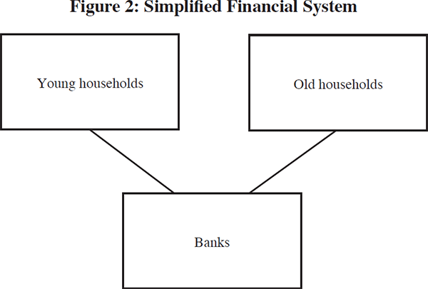
Our financial system has three groups – young households, old households and the banking sector (Figure 2). The only qualification to be a member of the financial system is to have a balance sheet. In this sense, households are fully-fledged constituents of the financial system.

The sole real asset that underpins the financial system is residential property. The young households hold part of the residential housing stock financed by borrowing from the banks. The young households thus have a particularly simple balance sheet (Figure 3, top panel). Their assets consist of property, while their liabilities consist of mortgages and net worth (if any).

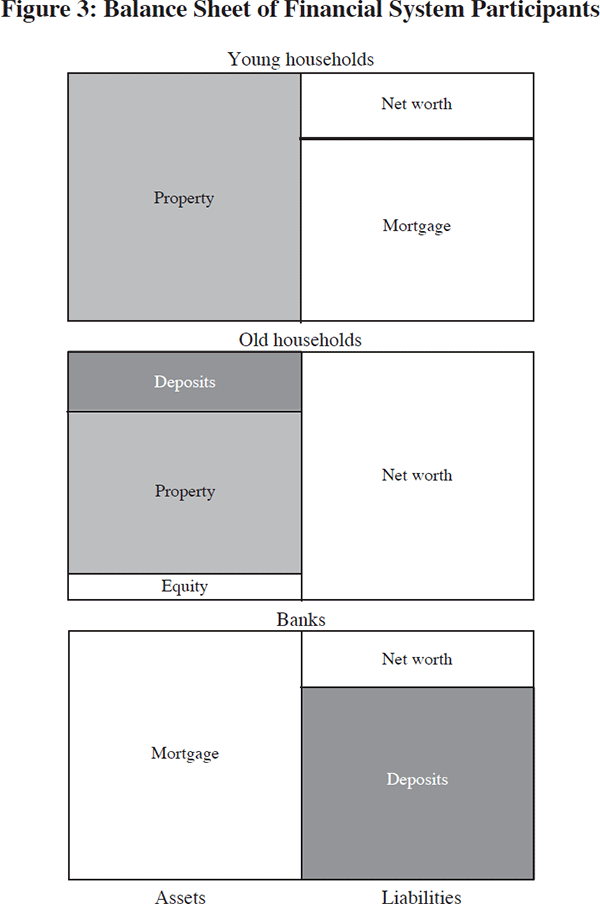
From the banking sector's point of view, the mortgage liabilities of the young households are its assets. The banks finance their lending through deposits of the old households. The contractual features of the deposit contract do not play a role in my argument, but it is important that banks' liabilities are of shorter duration than their assets. For my purposes, it is better to think of deposits as short-term claims on the banks. The balance sheet of the banking sector can be depicted as in the bottom panel of Figure 3. Old households hold residential property, deposits in the banking system, and are the equity holders of the banks themselves. They have no liabilities to other parties in the financial system, so that the whole of the liabilities side of their balance sheet consists of net worth (middle panel, Figure 3).

3.1 Duration difference in assets and liabilities

As I have described already, the contractual features of the deposit contract (such as the demandable nature of deposits) are not crucial for my story, but it is important that the marked-to-market value of deposits is less sensitive to long-term interest rates than the marked-to-market value of mortgage claims.

For simplicity, let us suppose that the treasury yield curve is flat, and that monetary policy works through parallel shifts of the yield curve. In this setting, a loosening of monetary policy induces a downward shift in the yield curve, raising both the value of deposits and mortgages. However, the value of mortgages rise by a larger proportion, reflecting their longer duration. Figure 4 illustrates the effect of monetary policy on the prices of mortgages and deposits. The relationships in Figure 4 are depicted in terms of straight lines, but this should not be taken literally. Among other things, mortgages may have embedded option elements such as early repayment. What is important is the fact that one unit of mortgage claims and one unit of deposits that start out with the same market value will diverge in value as monetary policy is either loosened or tightened.

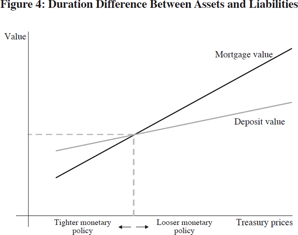
The banking sector holds mortgages on the asset side and deposits on the liabilities side. Thus, any shift in interest rates has a differential impact on its assets and liabilities. When monetary policy is eased, mortgage values rise by more than the value of deposits, raising the net worth of the banking sector, and reducing its leverage. Crucial to my story is the reaction of the banking sector to the increase in net worth. I will suppose that the banks react to the increase in net worth by increasing lending to the young households. The increase in lending could be quite moderate – for instance, the leverage of the banks could still be lower than before the fall in interest rates. However, the assumption is that the banks do not sit still when they see an increase in their net worth. The more accountable are the banks' management to their shareholders, and the more responsive they are to short-term incentives, the more likely it is that the banks will attempt to increase their lending.

I will assume that the banks can always find young households that are willing to borrow in order to finance the purchase of property, and that they (the banks) can find old households that are willing to lend to them in the form of greater deposits. Thus, from the point of view of the banks, they can always increase the size of their balance sheets by borrowing from old households and lending the proceeds to the young households.

The upshot of my assumptions on the behaviour of banks is that an increase in banking sector net worth resulting from the loosening of monetary policy results in a net flow of funds into the property sector, via the banks' balance sheets.

3.2 Property prices

An important part of my story is that the greater allocation of funds into the property sector leads to an increase in property prices. Let us suppose that there is an upward-sloping supply curve for property from the old households so that as bank lending to the young households increases, the price of the marginal property increases. Figure 5 depicts the upward-sloping supply curve. The implicit assumption is that there is some heterogeneity in the preferences of old households for housing services (which leads to the gradual increase in housing supply as the price rises), and that young households (as a group) place a higher value on housing than the old households. These differences may reflect, among other things, differences in remaining lifespans. Even if the per-period consumption value of housing were the same, younger households have longer to live, and hence may place a higher subjective value on owning the house, reflecting the higher capitalised value of housing services.

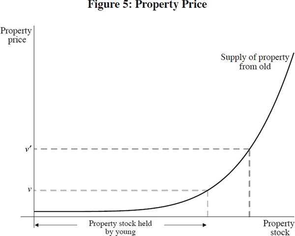
Figure 5 also illustrates the nature of property wealth in a financial system. The marked-to-market value of the housing stock increases in proportion to the price of the marginal-traded property. Does this mean that the net wealth of the economy has increased by the amount of the increase in the marked-to-market value of the housing stock? In our framework the answer would be ‘no’, since the increased property price simply reflects the marginal rate at which housing is reallocated from the old to the young. We have simply moved from one point in an Edgeworth box to another, rather than seeing an expansion of the Edgeworth box.

Bringing the various elements of the story together, we can now trace the impact of the strengthening balance sheet of banks on property prices. Denote the market price of mortgage claims as p, and suppose that monetary policy is eased, resulting in p rising by a greater proportion than the marked-to-market value of deposit liabilities. Monetary easing results in an increase in the net worth of the banking sector, inducing an increase in lending to young households (financed by greater deposits from old households). The young households then enter the property market with the new funds, raising the price of the marginal-traded property. Denote the price of property as v. Thus, an increase in the mortgage price p is associated with an increase in property price v. We can thus define v(p) as the price of property that is consistent with mortgage price p. Figure 6 illustrates the derivation of this relationship.

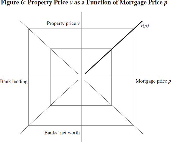
The bottom-right-hand quadrant indicates that as the mortgage price rises, banks' net worth increases. The bottom-left-hand quadrant is the key. It illustrates our assumption that as banks' net worth increases, banks are induced to increase their lending to young households. The top-left-hand quadrant shows the increasing relationship between bank lending and the price of property. This sequence of implications enables us to derive the curve v(p) that gives the property price as a function of the mortgage price.

4. Feedback

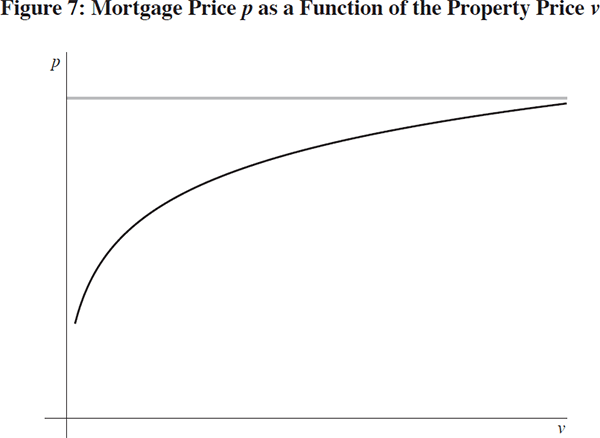
As the property price increases, the net worth of the household borrowers who have invested in property increases. To the extent that the loans to the household sector are collateralised against property, the rise in the property price raises the credit quality of the mortgage claims held by the banks against the young households, raising the marked-to-market value of the mortages held on the asset side of the banks' balance sheets.

Thus, we can define the price of mortgages, p(v), that is consistent with property price v. The price of mortgages is an increasing function of the price of property. Figure 7 illustrates this relationship. Since the increase in p is due to the increasing value of the assets that back the mortgage, there is an upper bound to p given by the price of the risk-free counterpart to the mortgage. This upper bound is indicated by the grey line.

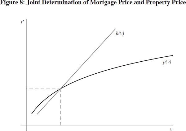
We can now bring the ingredients together to examine how the price of property interacts with the price of mortgages. Let us define h(.) as the inverse of the function v(p). Thus, h(v) is the mortgage price p that would give rise to price v of property. Plotting h(v) and p(v) on the same figure, we can derive the combination (v,p) of property price and mortgage price that would be mutually consistent. This is indicated in Figure 8.

With this framework, we can conduct some comparative statics with respect to some of the key quantities. Consider the effect of looser monetary policy that shifts the treasury yield curve down (Figure 9).

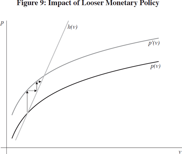
As monetary policy is eased, the yields on treasuries decline, inducing an upward shift in the price of mortgages that is consistent with the rise in treasury values (taking into account the assumed credit risk of mortgages). This initial movement is indicated by the left-most upward-pointing arrow following the upward shift in the p(v) curve. However, this initial change sets off a response from the property market. The higher price of mortgages strengthens the banks' balance sheets, and this in turn induces an increase in credit to young households. The proceeds of the increased loans end up in the property market, driving up the price of property. This second-round effect is indicated by the horizontal arrow pointing right, indicating an increase in v, the price of property.

The knock-on effects then propagate through the financial system. The second-round increase in v feeds through to higher credit quality of mortgages, which induces a further increase in the price of mortgages. This is indicated by the second vertical arrow, representing an increase in the price of mortgages. In turn, this induces a further increase in property prices, and so on. The financial system finds its new equilibrium where the higher p'(v) curve meets the h(v) curve. Depending on the slopes of the two curves, the eventual impact of the easing of monetary policy can be substantial.

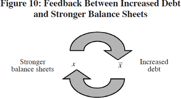
In terms of the framework of Section 2, the step adjustment mechanism depicted in Figure 9 can be seen as the feedback from the market value of claims (given by x) to the face value of claims (given by x). The market value of claims determines the strength of the marked-to-market balance sheets of the banks, and this influences the banks' lending policy. In turn, the increased lending flows into the property sector, raising property prices and mortgage values, thus influencing the market value of claims (Figure 10). I shall comment at the end of the paper on how this feedback mechanism may have been reinforced by recent developments in corporate governance and accounting regimes.

5. Reversal

The amplified response to the easing of monetary policy, by itself, need not be a problem for policy-makers if they can fine-tune their monetary policy levers to take account of the amplification. The problem would be rather like learning how to control the temperature of an unfamiliar shower by learning to turn the knob by the correct amount, and learning how quickly the water temperature reacts to turns of the knob.

Rather, the problem is the highly asymmetric nature of the mechanisms at play ‘on the way up’ versus the mechanisms ‘on the way down’. If the bursting of the property bubble impairs the solvency of the banking sector as a whole, then the dynamics ‘on the way down’ are likely to involve a whole new set of mechanisms that did not figure in the inflating of the bubble. These new mechanisms – default, distressed selling, and inefficient liquidations – are likely to conspire to exact very large economic costs.

Before turning to these new mechanisms, it is illuminating to see how far we can take the amplifying channels sketched above (that are responsible for the inflating of the property bubble) in explaining the reversal. Figure 11 illustrates the argument.

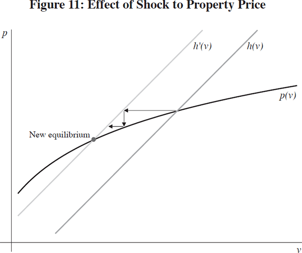
Starting from the initial intersection of the h(v) curve and the p(v) curve, let us trace through the impact of an exogenous fall in the property price, as represented by the leftward shift in the h(v) curve. The right-most horizontal arrow pointing left is the initial fall in property price. This fall in property price lowers the equity value of households, and so lowers the marked-to-market value of the mortgage assets held by the banks, leading to a fall in p. This fall in p is represented by the vertical arrow pointing downwards in Figure 11. The fall in p then lowers the banks' net worth, and the banks would respond by cutting back their lending to households. In our simplified model, the banks would have to foreclose on lending to some households, but this is due to the static nature of the model. In a dynamic model, the retrenchment of the banks would be manifested in the reduced flow of new lending to households. The reduction in the funds supporting the property market leads to a fall in the property price v. The feedback mechanism that was responsible for the amplified reaction of the property price then kicks into reverse gear. The credit quality of the collateral assets backing the mortgage declines further, leading to a further fall in the mortgage price, which then translates into less funds devoted to the property sector, and further falls in the property price. The system comes to rest at the new intersection point where both the property price and the bond price are considerably lower than their initial values. Depending on the relative slopes of the two curves, the eventual impact of a fall in asset prices can be very substantial.

5.1 New mechanisms

The story of reversal I have sketched above has important missing elements. New mechanisms will kick in ‘on the way down’ that did not figure in the process ‘on the way up’. In order to illustrate these new mechanisms, let us modify the story drastically by supposing that the banks hold property directly on their balance sheets, and that they mark their holding of property to market. Neither of these assumptions is appropriate in normal times, but they are a good approximation of an economy in the aftermath of the bursting of a property bubble where defaulting borrowers have handed property assets back to the banks, so that the banks end up holding the property directly. The balance sheet of a bank looks as in Figure 12.

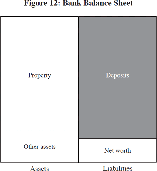
Assume that the assets held by a bank attract a regulatory minimum capital ratio, which stipulates that the ratio of the bank's capital – here taken to be simply the ratio of its marked-to-market net worth to the marked-to-market value of its assets – must be above some pre-specified ratio r^*. When a bank finds itself violating this constraint, it must sell some of its assets so as to reduce the size of its balance sheet.

I should emphasise that, although this constraint is expressed in regulatory terms, any bank that operates an internal risk management system will follow prescriptions that are similar to those expressed by the regulatory constraint. Under this alternative interpretation, the minimum ratio r^* could be much higher than the bare regulatory minimum.

I continue to denote the price of property as v. Let us denote bank i's holding of property by e_i, its holding of liquid assets by c_i, and its liabilities by l_i. It would be straightforward to extend this framework to take account of interbank claims along the lines discussed in Section 2 (see also Cifuentes, Ferrucci and Shin 2005). If we denote by s_i the amount of property sold by bank i, and by t_i the sale by bank i of its liquid assets, the capital adequacy constraint can be expressed as follows.

The numerator is the (marked-to-market) equity value of the bank while the denominator is the marked-to-market value of its assets after the sale of s_i units of property and sale t_i of the liquid assets. The underlying assumption is that the assets are sold for cash, and that cash does not attract a capital requirement. Thus, if the bank sells s_i units of property, then it obtains vs_i of cash, and holds v(e_i − s_i) worth of property. Hence, we have the sum of these (given by ve_i) on the numerator, while we have only the marked-to-market value of post-sale holding of property (given by v(e_i − s_i)) on the denominator. By selling its assets for cash, the bank can reduce the size of its balance sheet, reduce the denominator in the capital-to-asset ratio, and thus exceed the minimum capital asset ratio.

By re-arranging the capital adequacy condition (2), together with the condition that s_i is positive only if t_i = c_i, we can write the sale s_i as a function of v. If the capital adequacy ratio can be met by sales of liquid assets or from no sales of assets, then s_i = 0, but otherwise is given by

Thus, the sale of property s_i is itself a function of v, and we write s_i(v) for the sales by bank i as a function of the price v. Let be the aggregate sale of property by the banking sector given price v. Since each s_i(.) is decreasing in v, the aggregate sale function s(v) is decreasing in v.

I will now suppose that sales of property by banks can be absorbed by other constituents in the economy, provided the price is low enough. To give form to this idea, suppose that there is an exogenous demand function for property given by d(v). In my story sketched earlier, the old households would have a price at which they would be willing to buy back property. An equilibrium price of property is a price v for which

An initial shock to the property price may have an amplified response if the additional sales of property cause the price to fall further. The argument is illustrated in Figure 13.

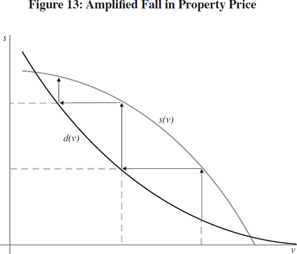
Consider a shock to the property price. The price adjustment process can be depicted as a step adjustment process in the arc below the s(v) curve, but above the d(v) curve. The process starts with a downward shock to the price of property. At the new lower price, the forced sales of the banks place a quantity of property on the market as indicated by the s(v) curve. However, the additional supply of property pushes the property price down, as implied by the d(v) curve. When the banks' balance sheets are evaluated at this lower price, the capital adequacy constraint may be violated, forcing yet more sales. The second-round supply of property is implied by the s(v) curve at the lower price. Given this increased supply, the price falls further, and so on. The price falls until we get to the nearest intersection point where the d(v) curve and s(v) curve cross. Equivalently, we may define the function Φ as

and an equilibrium price of property is a fixed point of the mapping Φ(.). The function Φ(.) has the following interpretation. For any given property price v, the value Φ(v) is the market-clearing price of property that results when the price of property on the banks' balance sheets is evaluated at price v. Thus, when Φ(v)<v, we have the pre-condition for a downward spiral in the property price, since the price that results from the sale of property is lower than the price at which the balance sheets are evaluated.

The lessons here are quite general. Changes in asset prices may interact with externally imposed solvency requirements or the internal risk controls of financial institutions to generate amplified endogenous responses that are large relative to any initial shock.

Regulators are familiar with the potentially destabilising effect of solvency constraints in distressed markets. To take one recent instance, the decline in European stock markets in the Northern summer of 2002 was met by the relaxation of various solvency tests applied to large financial institutions such as life insurance firms. In the UK, the usual ‘resilience test’ applied to life insurance companies in which the firm has to demonstrate solvency in the face of a further 25 per cent market decline was diluted so as to pre-empt the destabilising forced sales of stocks by the major market players.^[7]

More generally, the importance placed on asset prices follows the recent theoretical literature on banking and financial crises that has emphasised the limited capacity of the financial markets to absorb sales of assets (see Allen and Gale 2004, Gorton and Huang 2004, and Schnabel and Shin 2004), where the price repercussions of asset sales have important adverse welfare consequences. Similarly, the inefficient liquidation of long assets in Diamond and Rajan (2005) has an analogous effect. The shortage of aggregate liquidity that such liquidations bring about can generate contagious failures in the banking system.

6. Changing Nature of Monetary Policy

I conclude this paper by addressing myself more squarely to the theme of this year's RBA conference by drawing attention to a number of trends that have served to sharpen the effects outlined in my paper. In doing so, it is helpful to draw on the framework outlined in Section 2. There, I described the feedback between the strength of balance sheets (as implied by x) and the level of debt (as given by ). Strong balance sheets induce banks to increase their lending. In turn, increased lending raises property prices, leading to stronger balance sheets. Figure 14 depicts the feedback, and has labelled the possible forces at work in strengthening the feedback.

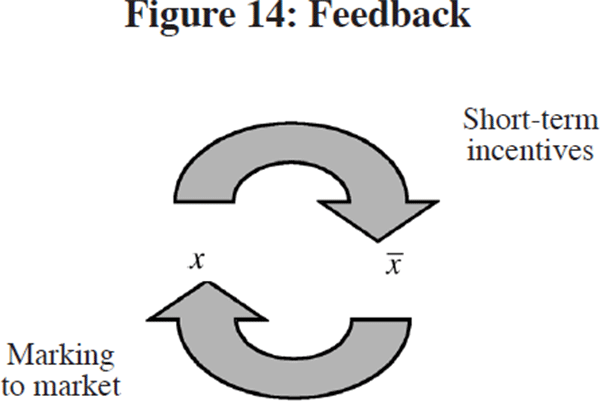
The reason why banks would increase their lending in the face of stronger balance sheets would be intimately tied to the short-term incentives facing the banks' management. Stronger balance sheets imply a larger marked-to-market value of equity for the bank. Suppose for the moment that shareholder value is measured in terms of return on marked-to-market equity (I return to this below). The more conscious is a bank's management to shareholder returns, the greater will be the incentive to react to the erosion of leverage by trying to restore leverage to some extent.

Indeed, the trend in recent years towards improved corporate governance through greater transparency, greater accountability to shareholders and greater use of incentive schemes tied to the share price will all strengthen the motives of the management to restore leverage. Whether such a move is actually in the interests of shareholders is a moot point (time horizons are the key). However, in a second-best world with many-layered agency problems, the shareholders would not wish to water down such short-term incentives.

What about the arrow going in the other direction – from increased debt (given by ) to stronger balance sheets (given by x)? The issue is how quickly the increased indebtedness translates into higher property prices and how quickly the increase in property prices is reflected in visibly stronger balance sheets. Here, marking to market is the key. For the US, the prevalence of mortgage-backed instruments as the prime source of finance for the property sector means that this pre-condition is already in place. For those economies that rely on bank lending, the accounting regime will be important. When assets and liabilities are marked to market continuously, the accounting numbers mirror the underlying market prices immediately.

Accounting numbers serve an important certification role in financial markets. They are audited numbers that carry quasi-legal connotations in bringing the management to account. As such, accounting numbers serve as a justification for actions. If decisions are made not only because you believe that the underlying fundamentals are right, but because the accounts give you the external validation to take such decisions, then the accounting numbers take on great significance.

To date, a thorough application of marking to market has affected only a small segment of the financial sector – notably, hedge funds and other hedge fund-like institutions that deal mainly with marketable claims. Marking to market has been limited by the lack of reliable prices in deep and liquid markets for many assets. Loans, for instance, have not been traded in large enough quantities to mark the loan book to market in a reliable way.

However, all this is about to change. The advent of deep markets in credit derivatives has removed the practical barriers to marking loans to market. The price of a credit default swap can be used to price a ‘notional’ loan corresponding to its standardised characteristics, much like the price of a futures contract on a bond, which indicates the price of a notional bond. Feasibility is no longer a hurdle to a thorough-going application of marking to market (or will not remain a hurdle for long).

It can be argued that mark-to-market accounting has already had a far-reaching impact on the conduct of market participants through those institutions that deal mainly with tradable securities, such as hedge funds and the proprietary trading desks of investment banks. However, even these developments will pale into insignificance compared with the potential impact of the marking to market of loans and other previously illiquid assets.

Accounting numbers, such as return on equity, have traditionally made reference to book equity (the accumulated value of past profits) rather than the market price of equity claims. However, this distinction is becoming increasingly less relevant. The recent trend (as prescribed by the new accounting standards) is to feed any capital gains to the profit and loss account (the income statement) so that capital gains and losses will be reflected immediately on the balance sheet.^[8]

Taken together, the increased reliance on short-term incentives and the greater immediacy given by marking to market hold huge significance for the conduct of monetary policy. I opened this paper by noting that monetary policy works by manipulating asset prices, especially long-term interest rates. The orthodox view of monetary policy is that, although the central bank generally directly controls only the overnight interest rate, it can nevertheless manipulate long-term interest rates since long-term rates are determined by expectations of the future course of short-term rates (modified by the appropriate risk premium). By charting a path for future short rates, and communicating this path clearly to the market, the central bank can control long-term rates. Having thus gained control of long-term rates, monetary policy works through the IS curve – through quantities such as consumption and investment.

This view of monetary policy reflects the origins of today's macroeconomics in the IS-LM view of the world, except for the fact that the ‘LM’ part has now been discarded. We have ended up with an exclusively ‘IS’ view of the world. In this world, financial markets play only a passive role, populated with far-sighted but essentially passive agents. It is a moot point whether such a view of financial markets was ever valid, but it is becoming evident that it is less of a good approximation today. Fed Chairman Alan Greenspan's ‘conundrum’ as to why long rates are so low today is a symptom of the breakdown of this view of markets.

When fixed-income traders and hedge funds trade 10-year swaps, are they influenced primarily by their forecasts of the future path of the fed funds rate over the next 10 years? Perhaps. What is clear is that there will be other shorter-term considerations that enter into their calculations. Understanding these considerations and heading them off will become an increasingly important part of monetary policy. The distinction between monetary policy and policies towards financial stability are perhaps less clear-cut than is supposed.

Footnotes

I am grateful to the discussant, Peter Westaway, and other participants at the conference for their comments. I thank Charles Goodhart and Raghu Rajan for their comments on an earlier draft. I am grateful to the IMF Research Department for its hospitality during the Northern summer of 2005 while this paper was prepared, and to the United Kingdom Economic and Social Research Council for its support under research grant RES-156-25-0026 as part of the World Economy and Finance programme. [1]

The conference volume from the Reserve Bank of Australia's 2003 conference gives a good snapshot of the state of the arguments at the time (see Richards and Robinson 2003). [2]

Official publications express these worries in more guarded terms. See Bank of England (2004a, 2004b) and IMF (2005a, 2005b). [3]

‘Mr. Greenspan's Cappuccino’ commentary by Brian S Wesbury, Wall Street Journal, 31 May 2005, p A16. The title makes reference to Alan Greenspan's comments on the ‘froth’ in the US housing market. [4]

Plantin, Sapra and Shin (2004, 2005) discuss other dimensions of the trade-off between marking to market and historical cost accounting. [5]

F is an increasing function of x on the complete lattice , and so has a largest and smallest fixed point by Tarski's fixed point theorem. Uniqueness follows from the fact that everywhere. The fact that x is increasing in follows from results on the comparative statics on lattices (Milgrom and Roberts 1994). See Shin (forthcoming) for proofs of all results reported here. [6]

FSA Guidance Note No 4 (2002), ‘Resilience test for insurers’. See also FSA Press Release No FSA/PN/071/2002, ‘FSA introduces new element to life insurers resilience tests’, 28 June 2002. [7]

Plantin et al (2004, 2005) discuss these and related issues. [8]

References

Allen F and D Gale (2004), ‘Financial intermediaries and markets’, Econometrica, 72(4), pp 1023–1061.

Bank of England (2004a), Financial stability review, June. Available at <http://www.bankofengland.co.uk/publications/fsr/2004/fsr16.htm>.

Bank of England (2004b), Financial stability review, December. Available at <http://www.bankofengland.co.uk/publications/fsr/2004/fsr17.htm>.

Bernanke BS (2002), ‘Asset-price “bubbles” and monetary policy’, remarks before the New York Chapter of the National Association for Business Economics, New York, 15 October. Available at <http://www.federalreserve.gov/boarddocs/speeches/2002/20021015/default.htm>.

Bernanke BS and A Blinder (1988), ‘Credit, money and aggregate demand’, American Economic Review, 78(2), pp 435–439.

Bernanke BS and M Gertler (1989), ‘Agency costs, net worth, and business fluctuations’, American Economic Review, 79(1), pp 14–31.

Borio C and P Lowe (2002a), ‘Assessing the risk of banking crises’, BIS Quarterly Review, December, pp 43–54.

Borio C and P Lowe (2002b), ‘Asset prices, financial and monetary stability: exploring the nexus’, BIS Working Paper No 114.

Borio C and P Lowe (2004), ‘Securing sustainable price stability: should credit come back from the wilderness?’, BIS Working Paper No 157.

Cifuentes R, G Ferrucci and HS Shin (2005), ‘Liquidity risk and contagion’, Journal of the European Economic Association, 3(2–3), pp 556–566.

Diamond D and R Rajan (2005), ‘Liquidity shortages and banking crises’, Journal of Finance, 60(2), pp 615–647.

Gorton G and L Huang (2004), ‘Liquidity, efficiency, and bank bailouts’, American Economic Review, 94(3), pp 455–483.

International Monetary Fund (IMF) (2005a), Global financial stability report, April. Available at <http://www.imf.org/external/pubs/ft/GFSR/2005/01/index.htm>.

IMF (2005b), World economic outlook, April. Available at <http://www.imf.org/external/pubs/ft/weo/2005/01/index.htm>.

Kashyap A and J Stein (2000), ‘What do a million observations on banks say about the transmission of monetary policy?’, American Economic Review, 90(3), pp 407–428.

Kiyotaki N and J Moore (1998), ‘Credit chains’, working paper, London School of Economics. Available at <http://econ.lse.ac.uk/staff/kiyotaki/creditchains.pdf>.

Kiyotaki N and J Moore (2001a), ‘Liquidity and asset prices’, working paper, London School of Economics. Available at <http://econ.lse.ac.uk/staff/kiyotaki/liquidityandassetprices.pdf>.

Kiyotaki N and J Moore (2001b), ‘Liquidity, business cycles, and monetary policy’, working paper, London School of Economics. Available at <http://econ.lse.ac.uk/staff/kiyotaki/liquiditybuisnesscyclesandmonetarypolicy.pdf>.

Kohn D (2005), ‘Imbalances in the U.S. economy’, remarks at the 15^th Annual Hyman P Minsky Conference, Levy Economics Institute of Bard College, New York, 22 April. Available at <http://www.federalreserve.gov/boarddocs/speeches/2005/20050422/default.htm>.

Merton R (1974), ‘On the pricing of corporate debt: the risk structure of interest rates’, Journal of Finance, 29(2), pp 449–470.

Milgrom P and J Roberts (1994), ‘Comparing equilibria’, American Economic Review, 84(3), pp 441–459.

Plantin G, H Sapra and HS Shin (2004), ‘Marking-to-market: panacea or Pandora's Box?’, working paper, London School of Economics. Available at <http://www.nuff.ox.ac.uk/users/Shin/working.htm>.

Plantin G, H Sapra and HS Shin (2005), ‘Marking-to-market, liquidity and financial stability’, paper presented at the 12^th International Conference hosted by the Institute for Monetary and Economic Studies, Bank of Japan, Tokyo, 30–31 May.

Richards A and T Robinson (eds) (2003), Asset prices and monetary policy, Proceedings of a Conference, Reserve Bank of Australia, Sydney.

Schnabel I and HS Shin (2004), ‘Liquidity and contagion: the crisis of 1763’, Journal of the European Economic Association, 2(6), pp 929–968.

Shin HS (forthcoming), ‘Credit risk in a system context’, London School of Economics.

Van den Heuvel SJ (2002a), ‘The bank capital channel of monetary policy’, Wharton School, University of Pennsylvania, mimeo. Available at <http://finance.wharton.upenn.edu/~vdheuvel/BCC.pdf>.

Van den Heuvel SJ (2002b), ‘Does bank capital matter for monetary transmission?’, Federal Reserve Bank of New York Economic Policy Review, 8(1), pp 259–265.