RDP 2013-12: Central Counterparty Links and Clearing System Exposures 5. Extensions

5.1 Non-normally Distributed Obligations

The analytical solution for R (Equation (4)) is based on the assumption that the distribution of obligations is normal. This solution may remain a fairly accurate approximation even if the assumption of normality is relaxed, provided that we retain the assumptions that the are identically distributed with finite variance and independent across i and j. These conditions allow the central limit theorem to be applied in estimating the distribution of default losses , which are based on the sums of the random variables .

Since , the central limit theorem implies that for a large N, the distribution of will be approximately normal, with mean zero and variance (N − 1)σ_k (as in Section 3), irrespective of the particular distribution of (provided they are independently and identically distributed with mean zero and a finite variance σ_k). The CCP's exposure to participant i will still be as in Equation (3), and the ratio R as in Equation (4), provided N is sufficiently large.

Symmetric, leptokurtic distributions that may be more appropriate for modelling financial returns include the Laplace (or double exponential) distribution and the t-distribution. Figure 8 compares the baseline analytical solution derived in Section 3 with the results of Monte Carlo simulations of the exposure ratio R for normal and non-normal distributions of (assuming zero correlation between product classes). Replacing the normal distribution for with a Laplace distribution or a t-distribution with 3 degrees of freedom (both finite-variance distributions) yields an exposure-netting ratio R that converges rapidly toward the analytical solution as N gets larger, as expected under the central limit theorem.

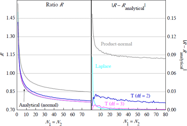
Relaxing the finite variance assumption, Figure 8 includes the case of the t-distribution with two degrees of freedom, as an example of a distribution with infinite variance. Under this distribution, the ratio R does not converge to the analytical solution, but remains slightly higher. However, the difference is sufficiently small as to be relatively insignificant in assessing whether or not CCP links increase or reduce aggregate CCP exposure.

The ‘product-normal’ case in Figure 8 relaxes the assumption of independence (and removes applicability of the central limit theorem), by decomposing the random variable for obligations, into the product of two random variables; , representing the size and direction of i's open position with j in product class k, and a price movement in product class k, Δp^k, which is common to all participants. In this example, it is assumed that both and Δp^k are distributed (0,1), with no correlation between k in either variable. The dependence across i and j now introduced between the means that the central limit theorem does not apply, with the ratio R remaining substantially above the analytical solution as N increases, although still falling below 1.

5.2 Multiple CCP Membership in the Linked Case

All of the previous analysis assumes that, once the two CCPs are linked, the N participants each consolidate their operations within one CCP only. While this would reduce participants' CCP membership costs, in reality participants may still choose to remain members of both CCPs even after interoperability is introduced.^[16] We now extend the model to account for this possibility. Let the number of participants, N, be divided into three categories:

• N′ participants who remain members of both CCPs, clearing product 1 through CCP1 and product 2 through CCP2, as in the unlinked case.
• N₁ participants who consolidate their operations in CCP1, clearing both products through that CCP.
• N₂ participants who consolidate their operations in CCP2, clearing both products through that CCP.

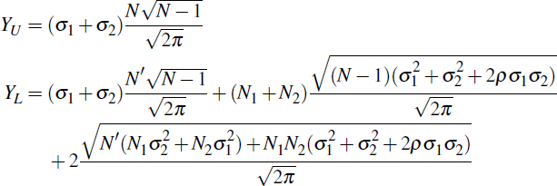
Accordingly, N = N′ + N₁ + N₂. Under the same assumptions discussed in Section 3, we obtain the aggregated unlinked and linked exposures:

Taking the base case of ρ = 0 and σ₁ = σ₂ yields

Figure 9 plots R for varying N′ as a proportion of N.^[17] The left edge of the graph (N′/N = 0) illustrates the case in which all participants consolidate their operations into either one of the two CCPs, as in Section 3. Accordingly, R is the same as previously. On the right edge of the graph, N′/N = 1, so that no participants change their operations. In this case, the link makes no difference because there is no change in the behaviour of the participants and no positions are put through the link. Therefore, R = 1.

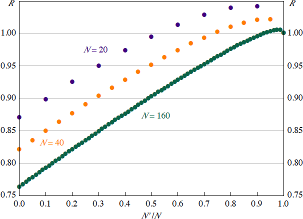
Generally, R increases with N′. Increasing N′ means that fewer participants choose to net their obligations in a single CCP, reducing netting benefits. Once N′ becomes sufficiently high, it is possible that R > 1. This occurs because most participants do not obtain any netting gain from the link. Further, for participants that consolidate their operations (say in CCP1), the majority of their trades in product 2 must be made in CCP2, because that is the venue for the majority of trades in product 2 made by the N′ participants. This means more of their trades are put through the link, which increases inter-CCP exposure.

5.3 Participant Heterogeneity

We have assumed so far that the have the same variance across all participant combinations i and j. This implies that all participants in each CCP pursue similar trading strategies with other counterparties, perhaps because they are of a similar size or have a similar level of appetite for risk. We now allow for a limited form of heterogeneity in , in which participants are either ‘large’ or ‘small’ in portfolio size or risk appetite (σ), and examine the effects in a two-CCP setting. This extension is particularly important in assessing cases such as that considered in Anderson et al (2013), where a smaller domestic CCP links to a larger foreign CCP. For CCP1, let there be ≤ N₁ ‘large’ participants, and similarly ≤ N₂ for CCP2. Let the ratio of standard deviations of values for ‘large’ and ‘small’ participants be g, such that:

Under this specification, trades between large participants involve additional variance, while the variance remains unaffected whenever a small participant is involved on either side of the trade. Assuming the X_ij are normally distributed, and letting N′ = + , we have:

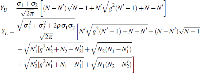
In the baseline case (σ₁ = σ₂, ρ = 0) this gives:

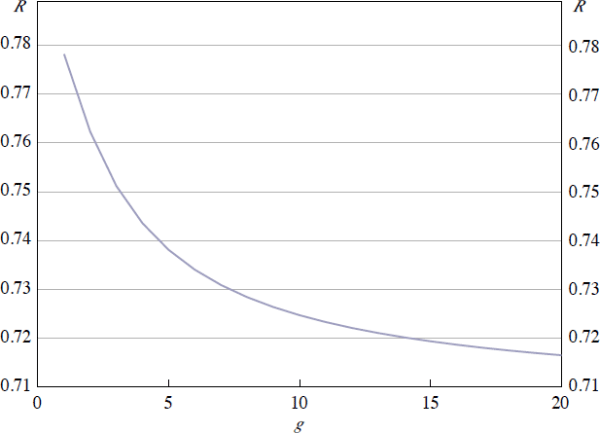
As in Section 4, we find that when participants are heterogeneous in this way, the asymmetry of activity across CCPs plays an important role in determining R, and works in a similar way to the asymmetry of participant numbers. We apply participant heterogeneity to the case examined by Anderson et al (2013), in which a domestic and foreign CCP establish a link. In the unlinked case, we let both N₁ domestic and N₂ foreign participants join both CCPs; they then consolidate their operations in the domestic CCP (CCP1) and the foreign CCP (CCP2) respectively.

Here, we consider a small jurisdiction in which all of the domestic participants are small on a global scale. All foreign participants are assumed to be large. We therefore have = 0 and = N₂. We now consider the effect of changing g, the ratio between the σ values for domestic and foreign participants. This is shown in in Figure 10 with N₁ = N₂ = = 50; increasing g lowers R. That is, increasing the asymmetry of activity across the two CCPs reduces the exposure arising from the link. This is because, given that m = σ₂/σ₁ is unchanged, the level of netting benefits across the two CCPs is the same. However, because a greater proportion of total activity takes place in the foreign CCP, the relative size of the inter-CCP exposures decreases. The net effect is that R decreases with the link.

5.4 Linking More than Two CCPs

We now extend the model to allow for link arrangements between C CCPs, where C > 2. In this section, we compare alternative arrangements for the netting of inter-CCP exposures: bilateral netting and multilateral netting through a meta-CCP, which acts as a CCP for inter-CCP exposures.

5.4.1 Bilateral netting

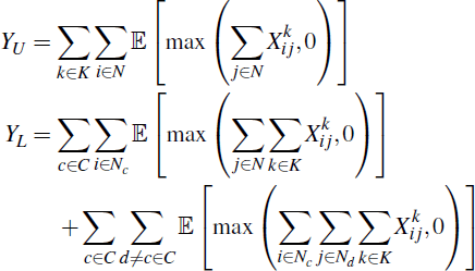
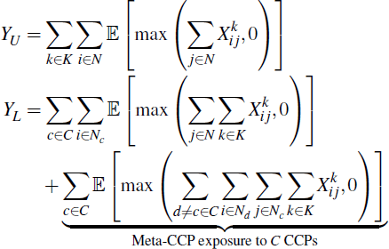
Let there be C CCPs that, in the unlinked case, clear a single product {1,…,K} respectively, and all K = C products once linked. Let N = Σ_c∈CN_c, where N_c is the number of participants that consolidate their operations in CCP c once the link is formed. If inter-CCP exposures are netted bilaterally, then the aggregate linked and unlinked CCP exposures are, respectively,

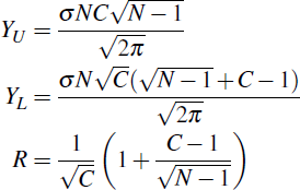
Let ρ_kl = Corr( , ). For simplicity, assume the base case of ρ_kl = 0 and σ_k = σ_l for all k and l. Further, assume membership is equally divided among the linked CCPs: N_i = = N/C. Assuming the are normally distributed yields:

As in Section 4, an increase in the total number of participants, N, increases R. As an example, the European CCPs LCH Clearnet Ltd, EuroCCP, EMCF and SIX x-clear have a four-way interoperability arrangement for many European cash equity markets. Taking the total number of participants in the linked CCPs, N = 105, we apply the base case of interoperability (equal σ_k values and ρ_kl = 0) to obtain R = 0.65. However, this result is heavily biased in favour of interoperability; in practice many clearing participants would be members of all four CCPs, to provide flexibility to their clients. As was shown in Section 5.2, maintaining multiple memberships after the link is formed results in a higher inter-CCP exposure, increasing R.

5.4.2 Multilateral netting

We could instead allow inter-CCP exposures to be multilaterally netted via a meta-CCP that takes on all inter-CCP obligations. Under this structure,

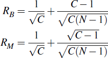
Taking the same base case as in Section 5.4.1, and letting R under bilateral and multilateral netting be R_B and R_M respectively, we have:

Since C > 2, R_M < R_B, indicating that link arrangements reduce exposure when inter-CCP exposures are multilaterally netted. Further, it can be shown that (R_B − R_M) is decreasing in N and increasing in C. Therefore, the additional benefits of multilateral netting fall when there are more participants, and increase when there are more linked CCPs. Taking the European example from the previous section (C = K = 4, N = 105), we have R_B = 0.65 and R_M = 0.54. As discussed previously, both these values are likely to be biased in favour of the link, but the difference between them nevertheless demonstrates the additional netting benefits of a meta-CCP arrangement.

Footnotes

In Europe, this has been driven by some participants having clients that prefer to clear with particular CCPs; continuing to clear on behalf of these clients requires participants to maintain multiple CCP memberships. [16]

Since N is constant and N = N′ + N₁ + N₂, the graphs show N′ increasing in increments of two, while N₁ and N₂ simultaneously decrease in increments of one. [17]