RDP 2013-09: Terms of Trade Shocks and Incomplete Information 2. A Small Open Economy Model
July 2013 – ISSN 1320-7229 (Print), ISSN 1448-5109 (Online)
- Download the Paper 941KB
The basic setup is a standard small open economy model with incomplete markets, similar to those in Mendoza (1995) and Aguiar and Gopinath (2007). I augment the model by assuming that agents are imperfectly informed about the contribution of permanent and transitory shocks to the observed terms of trade, requiring agents to solve a signal extraction problem.
In the model, households choose consumption, saving and labour supply to maximise lifetime utility. Households consume two goods – a good produced in their home economy, and an imported or foreign-produced good. The relative price of the two goods is the terms of trade, which is assumed to be exogenous to developments in the home economy. Households can invest in two assets – physical capital and a one-period non-contingent bond traded in international capital markets. The price of the bond is set exogenously, except for a small risk premium included to ensure that the economy's net foreign debt is stationary. There is one firm in the model, which features production with endogenous capital and labour. I augment the model with permanent and transitory productivity shocks and include capital adjustment costs. These features help the model to fit the data, but play little role in the analysis.
2.1 The Environment
2.1.1 Firms
The economy features a single perfectly competitive firm that produces a tradeable good using a Cobb-Douglas production technology of the form:

where Yt denotes output in period t, Kt denotes capital and Nt denotes hours worked. At and Xt are productivity shifters. The process, At, is stationary and follows a first-order autoregressive process in logs. In what follows, I use lower-case letters to represent log deviations from a variable's steady state, so that at = lnAt, − lnA* where A* is the steady state value of At. The evolution of at then follows:

The second productivity shock, Xt, is non-stationary. Let
I assume that the logarithm of Mt follows a first-order autoregressive process of the form:

The parameter μ measures the deterministic growth rate of the productivity factor Xt. The parameters ρa, ρm ε [0,1) govern the persistence of at, and mt. Somewhat loosely, I refer to at and mt as transitory and permanent productivity shocks, respectively.
Profit maximisation by the firm ensures that factor prices reflect marginal value products:
where Wt is the nominal wage,
 is the price of the home-produced good
and
is the price of the home-produced good
and
 is the rate of return to capital.
2.1.2 Households
Households maximise expected lifetime utility given by:
where β is the household's rate of time preference, Ct is consumption, Nt is hours worked, φ is the inverse of the labour supply elasticity and AL is a constant used to calibrate average labour supply in the model to match that in the data.
The household's consumption bundle is a Cobb-Douglas aggregate of home- and foreign-produced goods,
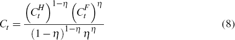
where
 are home-produced goods and
 are foreign-produced goods. The parameter
η ε (0,1) governs the relative weights of home- and foreign-produced
goods in the household's consumption bundle. Let Pt
be the consumer price index corresponding to Ct. Then,
are foreign-produced goods. The parameter
η ε (0,1) governs the relative weights of home- and foreign-produced
goods in the household's consumption bundle. Let Pt
be the consumer price index corresponding to Ct. Then,

where
 is the price of the foreign-produced
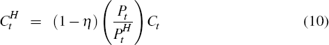
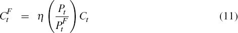
good. Household optimisation ensures that the demand for home- and foreign-produced
goods is given by:
is the price of the foreign-produced
good. Household optimisation ensures that the demand for home- and foreign-produced
goods is given by:
Households have access to two assets: domestic capital and a single-period, risk-free bond, denominated in the foreign good. The household's period-by-period budget constraint is:

where Qt denotes the price of one-period risk-free bonds, Bt+1 denotes the stock of bonds acquired in period t, It denotes gross investment and ϕ is a parameter that controls the cost of adjusting the size of the capital stock. The capital stock evolves according to the law of motion:

where δ ε [0,1) denotes the depreciation rate of capital.
To ensure that the solution to the model is stationary, I assume that the country faces a debt-elastic interest rate premium as in Schmitt-Grohé and Uribe (2003). Specifically,
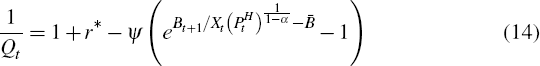
where r* is the exogenous foreign rate of interest on a risk-free
bond and  is the steady-state foreign asset level.
Household utility maximisation implies the following first order conditions:
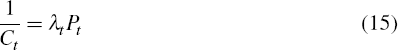

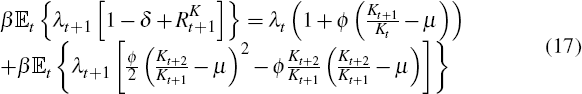

where λt is the Lagrange multiplier on the household's budget constraint.[5]
2.1.3 Relative prices
I take the price of the foreign good,
, as the numeraire and normalise it
to 1. I define the terms of trade, St, as the relative
price of home-produced goods in terms of foreign-produced goods. It follows
from the definition of the consumer price index that:
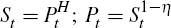
The home economy is assumed to be small in the sense that it is a price-taker on world markets. Consequently, changes in its terms of trade are exogenous to domestic variables. The terms of trade are assumed to follow the process,

The first component, Zt, represents a transitory shock to the terms of trade, which is assumed to follow a first-order autoregressive process in logs. That is,

The second component, Γt is a permanent terms of trade shock. Let,
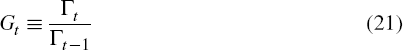
I assume that the logarithm of Gt follows a first-order autoregressive process of the form:

The decomposition of the terms of trade outlined in Equations (19)–(22) is
extremely flexible and encompasses many of the assumptions about the evolution
of the terms of trade used in other papers. For example, if
 = 0, the terms of trade is
subject to purely transitory shocks, while if
= 0, the terms of trade is
subject to purely transitory shocks, while if
 = 0 and ρg
= 0 then the terms of trade follows a random
walk.[6]
= 0 and ρg
= 0 then the terms of trade follows a random
walk.[6]
2.1.4 Market clearing
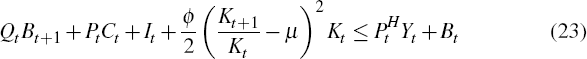
Market clearing requires that the quantity of goods produced in the home economy equals the consumption of these goods at home and abroad. This is ensured by the current account condition:
2.1.5 Equilibrium
An equilibrium is a sequence of quantities
 ,
prices
,
prices
 and exogenous processes
 such that
(i)
firms maximise profits, which implies Equations (5) and (6), (ii) households maximise
utility, which implies Equations (15)–(18), and (iii) markets clear,
given by Equation (23), subject to the technological and resource constraints
in Equations (1), (13), (14) and (19) and the exogenous processes given in
Equations (2), (4), (20) and (22).
such that
(i)
firms maximise profits, which implies Equations (5) and (6), (ii) households maximise
utility, which implies Equations (15)–(18), and (iii) markets clear,
given by Equation (23), subject to the technological and resource constraints
in Equations (1), (13), (14) and (19) and the exogenous processes given in
Equations (2), (4), (20) and (22).
2.2 Information Structure
I assume that agents have complete information about all aspects of the economy other
than the components of the terms of trade, about which they are imperfectly
informed. In particular, I assume that agents can observe the level of the
terms of trade but cannot observe Zt
or Γt directly. Reflecting the fact that agents are
likely to have some information about the persistence of these shocks, I assume
that agents receive a noisy signal regarding the permanent terms of trade shock.
I refer to this signal as ht such that ht
=
gt +
 where
are independently and identically distributed
with mean zero and variance
where
are independently and identically distributed
with mean zero and variance
 . The agents' information set as
of time t includes the entire history of terms of trade shocks and
signals;
. The agents' information set as
of time t includes the entire history of terms of trade shocks and
signals;
 ≡ {St,ht,S
t−1,ht−1,…}.
≡ {St,ht,S
t−1,ht−1,…}.
In the model, agents form expectations about the decomposition of the terms of trade using the Kalman filter. To implement this, I represent the agent's filtering problem in state space form using the decomposition in Boz et al (2011). First, I define the growth rate of the terms of trade as:
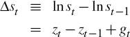
The measurement equation includes a reformulation of this definition as well as the definition of the noise process:
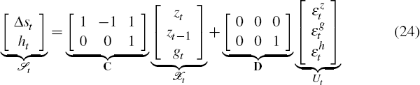
The transition equation summarises the evolution of the unobserved variables and is given by:
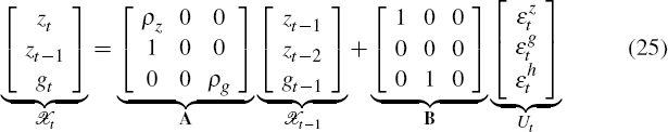
where
 .
.
The Kalman filter can then be used to express the consumers' beliefs about the components of the terms of trade in recursive form as:

where
 is an identity matrix and K
is the Kalman gain, calculated as:
is an identity matrix and K
is the Kalman gain, calculated as:

and L is the steady-state error covariance matrix, calculated as the solution to:

Equations (26)–(28) fully characterise learning.
2.3 Model Solution
I solve the model by taking a log-linear approximation to the equilibrium conditions
derived in the previous
section.[7]
The solution of the model follows Uhlig (1999) and Blanchard et al
(forthcoming). Let  t
denote the endogenous variables controlled by the agent. The economic model
can be represented as the stochastic difference equation:
t
denote the endogenous variables controlled by the agent. The economic model
can be represented as the stochastic difference equation:

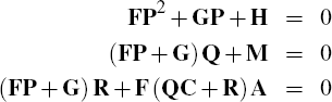
where F, G, H, M and N are matrices of parameters
and  t
is the vector of observable variables described in section 2.2.
The unique stable solution of the model is:
t
is the vector of observable variables described in section 2.2.
The unique stable solution of the model is:

where
 represents the agents' expectation
of the unobserved states described in section 2.2. The
matrices P, Q,
R can be found by solving the three matrix equations:
represents the agents' expectation
of the unobserved states described in section 2.2. The
matrices P, Q,
R can be found by solving the three matrix equations:
where the matrices A and C are as defined in Section 2.2.
Footnotes
Note that in taking first order conditions with respect to the foreign debt level, I have assumed that agents take the interest rate on foreign assets as given – that is, they do not internalise the effect of their decisions on their borrowing costs. For a discussion of the implications of internalisation of the risk premium, see Lubik (2007). [5]
The terms of trade will also follow a random walk if ρg
= ρz = ρ and
 .
[6]
.
[6]
Appendix B outlines the model's steady state and the log-linearised equations. [7]