RDP 2012-07: Estimates of Uncertainty around the RBA's Forecasts 2. Data

Uncertainty about a forecast can be gauged by the performance of similar forecasts in the past. To this end, it would be desirable to have a record of forecasts resulting from a similar process applied to similar information sets. In practice, processes and datasets have evolved over time. For example, the SMP has only recently included numerical forecasts for inflation and GDP. In the earlier part of our sample, we use internal forecasts prepared by the RBA staff, which we assume have similar properties to those published in the SMP. At the risk of over-simplifying, we refer to all these forecasts as ‘RBA forecasts’ even though many of them have little official status.

We discuss our data in detail in Appendix B. However, a few important features are worth noting here. Our sample extends from 1993:Q1, when inflation targeting began, through to 2011:Q4. We try to measure actual outcomes with definitions close to those used in the forecast. For GDP growth, this means using near-real-time data, while for underlying inflation we use definitions used at the time of the corresponding forecast.

We show some illustrative data in Figure 1. The dark lines in the top half of each panel represent actual outcomes, measured with near-real-time data, for underlying inflation, the CPI, real GDP growth and the unemployment rate. The light lines in the same panels represent the forecasts of these variables from three quarters earlier. For series published with a one quarter lag, this horizon encompasses the first four quarters of data.^[1]

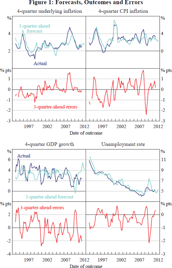
One (of many) interesting features of Figure 1 is the differing explanatory power of forecasts for different variables. As can be seen in the top two panels, many of the variations in underlying and headline inflation were predicted in advance. In contrast, the relationship between the forecasts and GDP growth (third panel on left) is harder to see. We elaborate on this point below.

Figure 1 also presents 3-quarter-ahead forecast errors, measured as outcomes minus forecasts, shown in the bottom half of each panel. As might be hoped, the errors lack obvious patterns. With some exceptions, discussed below, they do not trend, they are centred on zero, they have little persistence (beyond that expected given the 3-quarter-ahead forecast horizon) and their variance does not change noticeably over time. Whereas many other countries experienced extreme adverse forecast errors during the recent global financial crisis, that did not happen in Australia.

Although the data are discussed in detail in Appendix B, one point worth noting here is that the forecasts are conditional on interest rate assumptions. For most of our sample, an unchanged cash rate was assumed. However, when this assumption seemed obviously unrealistic, as in the period following the global financial crisis, forecasts instead assumed a path broadly consistent with market expectations. Unless there is a change in procedures going forward, that assumption does not affect the construction of confidence intervals or other measures of uncertainty. Were this approach to change, it would probably have little effect on measures of forecast accuracy, as we discuss in more detail in Appendix B.

Footnote

These forecasts are for the current quarter and following three quarters, which we refer to as ‘first year’ or ‘3-quarter-ahead’ forecasts. Because the timing of the forecast differs from the timing of the most recent data, the common ‘h-period-ahead’ terminology is ambiguous. We measure horizons from the date of the forecast, which is convenient in dealing with variables with different release dates and publication frequency. A popular alternative convention is to measure horizons from the date of the latest data, in which case the forecasts and errors in Figure 1 would mainly be described as ‘4-quarter-ahead’. [1]