RDP 33 Inflation: Prices and Earnings in Australia II Theoretical Model
April 1974
In a decentralised market economy, decisions by firms and households are subject to constraints imposed by government. Both firms and households operate in all of the three main domestic markets; the goods market, the labour market and the money market. The equations developed in this paper are attempts to explain movements in prices in the goods and labour markets. As the objective of this paper is not to develop a general equilibrium model of the whole economy but rather to construct a partial equilibrium model capable only of examining prices and earnings, equations are not developed for the money market. However, the money market would be included in policy analysis if the price and earnings equations were incorporated in a complete model of the economy.
The theory is developed from the proposition that firms and households seek to maximise profits and utility respectively. Firms and households depend on one another; firms supply goods and demand labour while households supply labour and demand goods.[2] In the development of a theory of inflation, there is a need to take account of at least one fundamental difference between the labour and goods markets. Unlike labour, goods (like money) are highly mobile between different countries. Firms within a given country supply goods to local as well as overseas households while households usually supply labour only to local firms.[3] Whether a firm will supply goods to the local or the overseas market will, of course, depend at least partly on the relative prices offered. The decision of households to buy local or overseas goods will also depend partly on relative prices.
International arbitrage in the goods market will ensure that the prices of tradeable goods (defined as all goods and services with a potential to be traded; this incorporates a much wider range of goods than just those actually traded) in different countries adjusted for changes in exchange rates will broadly move together. The prices of non-tradeable goods (mainly services) in a particular country will be connected to the prices of tradeable goods by the price of labour and other inputs so that in the long-run, it could be expected that the prices of tradeable and non-tradeable goods will also broadly move together.[4]
These open economy considerations suggest that, in the short-run, there is a need to develop a theoretical model which explains separately the price of tradeable goods and the price of non-tradeable goods. These two price equations can then be used to give a joint explanation of prices in the total market for goods and services.
To re-capitulate: the theoretical model proposed attempts to describe the pricing behaviour in three markets; the labour market, the market for non-tradeable goods and the market for tradeable goods. Firms and households are the two decision-making economic agents operating in these three markets.
As shown in Appendix A, the following market demand and supply functions are consistent with a firm maximising profit, subject to a production function constraint, and a household maximising utility subject to a budget constraint.
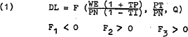
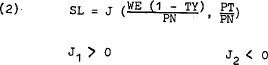
Labour market:
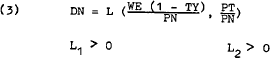
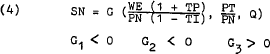
Non-tradeable goods market:
Tradeable goods market:
| where[5] | DL | – | demand for labour |
| DN | – | demand for non-tradeable goods | |
| DT | – | demand for tradeable goods | |
| PN | – | price of non-tradeable goods | |
| PT | – | price of tradeable goods | |
| Q | – | productivity (average output-labour ratio) | |
| SL | – | supply of labour | |
| SN | – | supply of non-tradeable goods | |
| ST | – | supply of tradeable goods | |
| TI | – | sales and other indirect taxes (as a rate) | |
| TP | – | payroll and related taxes (as a rate) | |
| TY | – | income taxes (as a rate) | |
| WE | – | average weekly earnings |
and the Fi, Ji etc. refer to the partial differential of the i-th argument of the functions F, J and so on.
All these functions are assumed to be homogeneous of degree zero in wages and prices. The demand for labour is expressed as a negative function of the real wage cost to firms (wages plus pay-roll taxes[6] divided by the price of non-tradeable goods after sales taxes) and as a positive function of the prices of both tradeable and non-tradeable goods as well as productivity. The elasticity of demand with respect to real wage cost would have to be greater than that with respect to the relative price term if the net elasticity on the price of non-tradeables is to be positive, as would conventionally be expected. Capital is not directly included in the demand function as the analysis is essentially short-run. However, any change in the capital-labour ratio would have an indirect effect on the demand for labour through the productivity term. The supply of labour function simply states that the supply will increase if after tax wages increase and prices of tradeable and non-tradeable goods decrease (again assuming that the supply elasticity with respect to the price of non-tradeables arising from the real wage term outweighs that from the relative price term).
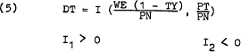
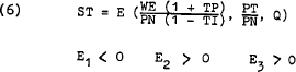
In the goods market, the demand for non-tradeable goods is expressed as a positive function of wages after income tax and the price of tradeable goods and a negative function of the price of non-tradeable goods. The supply function states that the supply of non-tradeable goods will decrease if wages (net of payroll taxes)and the prices received for tradeable goods increase and the supply will increase if the price of non-tradeables (after tax) and productivity increase. The domestic demand and supply functions for tradeable goods are the same as for non-tradeable goods with the exception that the sign on each of the price terms is reversed.
If excess demand (X) is defined as demand (D) minus supply (S) -

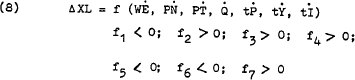
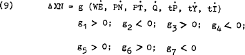
then the following dynamic excess demand functions can be derived for the labour market, the non-tradeable goods market and the tradeable goods market[7] –
| where | tI | = | 1 – TI (for notational convenience) |
| tP | = | 1 + TP (for notational convenience) | |
| tY | = | 1 – TY (for notational convenience) | |
| XL | = | excess demand for labour | |
| XN | = | excess demand for non-tradeable goods | |
| XT | = | excess demand for tradeable goods |
a dot over a variable indicates proportional rate of change and Δ indicates absolute change
The direction of causation implied by each of these behavioural equations as they stand at present is from the right hand side variables to each of the excess demand terms. That is, the independent variables form a set, exhausting all possible (or at least major) sources of shifts of and along the excess demand schedules. An important feature of these three equations is that from the point of view of the individual firms and households, from whose behaviour the specifications were derived, the right-hand side variables are truly independent, even though they are determined endogenously within the macro-economic system. This means that, if in say equation (8) the independently determined rate of change of wages decreases, or that of tradeable prices increases, then there would be a resulting increase in the excess demand for labour through the reactions of firms and households. However, this is not the whole story. At the aggregate level, the wage rate (and to a much lesser extent the other variables on the right-hand side of equation (8)) is not independent of conditions of supply and demand in the labour market. Rather, those who set or bargain for the money wage rate, do so in such a way as to eliminate excess demand. If at any point in time there is an excess demand for labour then the wage rate would need to be raised if the wage-setters wished to reduce or eliminate the excess (the negative relationship indicated in equation (8)).
In discrete periods of time the wage decision is more complex. In this analysis it is assumed that at the beginning of each period wage-setters decide how to adjust the wage rate so as to eliminate any excess demand or supply existing at the end of the previous period. In addition, they must decide if some further adjustment is required to eliminate expected changes in excess demand during the period. This latter source of change must necessarily arise from changes in one or more of the other variables on the right-hand side of equation (8) as those terms formed an exhaustive set of the sources of change in excess demand. As the wage-setters do not know with certainty how excess demand will behave over the period, they must set wages in accordance with excess demand existing at the end of the last period, taking account of their expectations of change in any of the other variables influencing excess demand during the period.
Thus a decision is made at the beginning of the period to set a wage level (and thus a rate of change of wages) such that the expected change in excess demand, accoounting for other expectations, offsets the level of excess demand existing at the end of the last period –
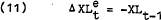
where superscript e denotes expected and subscript t indicates time period t. This implies that the expected level of excess demand in period t is zero. Excess demand does exist at the beginning of the period and at the end of the period to the extent that the wage-setters are unable to judge the exact relationship between wages and excess demand and to the extent that their expectations are incorrect.
Another way of describing this adjustment mechanism is to consider equation (8) in terms of labour market equilibrium over time. If the labour market is to be in equilibrium over time then the change in excess demand in each period must always be zero. That is, the functional rates of change of each of the terms on the right-hand side of (8) must sum to zero. As wages have been specified to react so as to clear the market, the equilibrium condition implies that the rate of change of wages perfectly offsets some additive function of all the other rates of change in (8). This can only occur if two conditions are met. The first is that the market is initially in equilibrium and the second that the changes in productivity, prices and taxes are perfectly anticipated so that in each decision period, wages are simply adjusted so as to offset them. Given that these two conditions are not met, but assuming that wage decisions are still made on a rational market clearing basis, a simple mechanism of wage movements can be specified.
Firstly, to account for the fact that the market is not continually in equilibrium it is hypothesised that wages adjust in each period not only so as to offset changes in the other determinants of excess demand but also to eliminate any excess demand that exists at the beginning of the period due to errors of judgment in previous periods. Then, to account for the absence of perfect knowledge it is hypothesised that in each decision period, wages are adjusted[8] so as to offset expected changes in the other determinants of excess demand as well as any excess demand existing at the beginning of the decision period. A reassessment is made at the beginning of each decision period according to new expectations and the errors involved in the last period. The non-coincidence of all decision-makers' time periods and of data and decision periods raises an empirical problem with this theoretical specification which will be discussed in a later section.
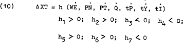
Equations (8) and (11) imply a behavioural equation for the rate of change of wages as a function of past excess demand and expectations with respect to the rates of change of prices, productivity and taxes[9] –
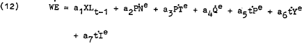
where a5 and a6 are expected to be negative. In the same way, it is argued that the producers setting prices in the non-tradeable goods market do so in such a way as to eliminate any existing and expected excess demand for their products. That is, the rate of change of the price of non-tradeables is set so that –
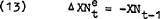
Equations (9) and (13) imply a behavioural equation for the rate of change of the price of non-tradeable goods as a function of past excess demand for non-tradeable goods and expectations with respect to the rates of change of wages, tradeable prices, productivity and taxes[10] –

where b4 and b7 are expected to be negative
With respect to tradeable goods, the market clearing mechanism is assumed to be slightly different. As pointed out earlier, tradeable goods, unlike labour and non-tradeable goods, are highly mobile between countries with the result that theoretically, for a small open economy the supply and demand for such goods would be perfectly elastic about any given price. The prevailing price would be the equilibrium world price for such goods, translated into a domestic equivalent via the exchange rate. In this way, an excess demand or supply of domestic tradeable goods occasioned by a change in one of the other exogenous variables would cause a quantity adjustment (through flows of imports or exports) rather than a price adjustment to clear the market. An attempt to set the price of tradeable goods at a level different to that prevailing in the rest of the world would bring about very large changes in excess demand pushing the general domestic level of tradeables back to the world level.
In other words, for a small open economy, the price of tradeable goods is approximately equal to the world price of tradeable goods adjusted for the exchange rate[11] –

and so
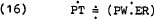
where PW is the world price of tradeable goods and ER is the effective exchange rate.
For a discrete period analysis, it is postulated that the rate of change of the price of tradeable goods is set at the beginning of each period in accordance with expectations about world prices and the exchange rate. That is –
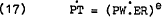
Equations (12), (14) and (17) form a consistent theoretical wage-price model, which can be estimated directly so long as suitable statistical series can be found or proxied for the excess demand and expectations terms.
Footnotes
For a useful analytical model outlining the interdependence of firms and households in the goods and labour markets, see Barro and Grossman [1]. [2]
The role of immigration in the labour market is an area of analysis receiving a recent revival of interest. For the purposes of this paper however international mobility of labour is assumed to be insignificant in its impact on the labour market. [3]
For a fuller discussion of the relationship between tradeable and non-tradeable goods and prices, see Johnson [6] and Caves [2]. [4]
A comprehensive list of all notation used in this paper is included in Appendix B. [5]
While pay-roll taxes are the major source of divergence between the real cost of wages to the firm and the real wages received by employees, they need not be the only source. This term could be expanded to include superannuation payments by employers and other costs of hiring labour. Likewise, other non-labour costs could be included in the indirect tax term. The restricted form of the profit function and budget constraint assumed in Appendix A avoids these other cost terms but this remains a weakness. [6]
These equations are specified in detail in equations A.39, A.54 and A.59 respectively of Appendix A. [7]
In this model a complete adjustment is hypothesised. In fact a partial adjustment mechanism based on an error-learning process or some other form of adjustment dynamics may be more appropriate. This is regarded as an important improvement to be taken up in later work. [8]
Where the signs are derived in detail in equations A.41 and A.42 of Appendix A. [9]
Again the signs and form are contained in Appendix A in equations A.56 and A.57. [10]
This behavioural approximation for tradeable prices is more correctly a long-run relationship and is an over-simplification in the short-run even for a fairly small open economy such as Australia's. This is a weakness of the current paper which will be rectified in following work. [11]