Introduction | RDP 33 Inflation: Prices and Earnings in Australia

RDP 33 Inflation: Prices and Earnings in Australia IV Prices

Peter Boxall and Jeff Carmichael

April 1974

This section attempts to test empirically the model of price behaviour suggested by equations (14) and (17). The construction of variables and formulation of the estimating equations will be dealt with in one sub-section, while a second sub-section will report and comment on the estimated results.

IV-I Empirical Constructions

It has already been observed that series are not available for either of the price sub-groups. This does not mean that estimates of price inflation cannot be produced. Rather, it means that the price sector has to be reduced to an analysis of aggregate price behaviour only. This can be achieved by making use of the proposition (foreshadowed in equation (22)) that the aggregate price level is a weighted sum of the prices of non-tradeable and tradeable goods. That is –

View MathML

Thus using the behavioural equations for the rates of change of the prices of non-tradeables (equation (14)) and tradeables (equation (17)) provides an unconstrained estimating form for the aggregate rate of price inflation –

View MathML

Imposing the constraints^[24] that –

b₂ + b₃	=	1
b₅ + b₆	=	b₂
and b₅	=	−b₇

gives –

View MathML

In the estimating forms, four quarter percentage changes are again used to represent rates of change and the expectations terms are each approximated by a distributed lag on current and past values. The excess demand term is the same as that used in the earnings equation; the main reason for this is the inability to construct a meaningful series for excess demand in the non-tradeable goods market.^[25]

IV-II Empirical Results

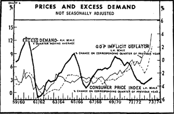
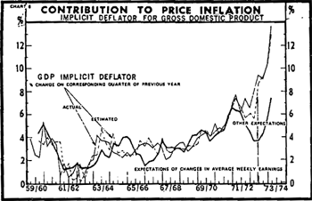
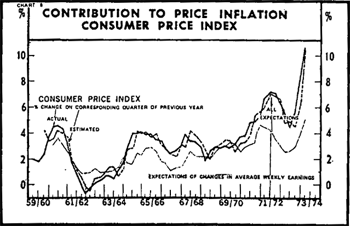
Equations are estimated for the implicit deflator for gross domestic product (PGDP) and the consumer price index (PCPI) using the estimating forms of equations (29) and (29). The data period is again 1960(1)–1973(3) and the results are reported in Table 2.^[26] The courses of excess demand (V*−U) and the rates of change of each of the price variables are graphed in Chart 4 and the relative contributions of expectations about average weekly earnings and the remaining terms to each of the two measures of price inflation are graphed in Charts 5 and 6.

Table 2
Price Equations 1960(1)–1973(3)
Equation	G	V*−U	(V*−U)₋₄							S.E.E.		D.W.		F
Equation (28.a) PGDP	1.083	−.269	−.110	.516	−.067	−2.759	−.613	.146	−.362	.980	.853	2.45	.729
Unconstrained	(0.6)	(1.4)	(0.6)	(4.2)	(0.3)	(1.5)	(2.5)	(0.2)	(3.1)
Equation (29.a) PGDP	−2.247	−.516	−.350	.801	.199	926	−.125	−.926	−.430	1.080	.828	2.00	.724	3.594
Constrained	(3.0)	(3.1)	(2.1)	(–)	(2.2)	(4.2)	(–)	(4.2)	(3.6)
Equation (28.b) PCPI	1.874	.098	−.066	.357	−.112	1.569	–.417	-255	−.232	.666	.896	1.69	.9
Unconstrained	(1.6)	(0.7)	(0.5)	(4.3)	(0.8)	(1.3)	(2.5)	(0.5)	(2.9)
Equation (29.b) PCPI	−1.268	−.107	−.304	.576	.424	.925	−349	−.925	−347	.769	.877	1.46	.9	4.289
Constrained	(1.2)	(0.8)	(2.3)	(–)	(6.1)	(5.9)	(–)	(5.9)	(4.2)
Notes: PGDP is the implicit deflator for gross domestic product and PCPI is the consumer price index. A dot over a variable indicates proportional rate of change (J4P). A superscript e indicates use of a second degree Almon variable to approximate an expected value. The value in brackets under the estimated coefficients are t values. A value greater than 1.960 indicates significance at the 5 per cent level. S.E.E. is the absolute standard error. The average value of PGDP is 4.032 per cent and that of PCPI 3.389 per cent. The D.W. statistic is a test for first order autocorrelation. P is the weight given to the lagged values in a Hildreth-Lu correction for first order autocorrelation. The F ratio indicates the validity of the constraints. A value less than 2.78 indicates acceptability at the five per cent level of significance and less than 4.16 at the one per cent level. Variables: are as in Table 1 with the exception of which is the expected rate of change of average weekly earnings (Almon on J4P) and the dependent variables which are the proportional rate of change of PGDP in equations (28.a) and (29.a) and the proportional rate of change of PCPI in equations (28.b) and (29.b).

Click to view larger

The empirical price equations do not provide good support for the theoretical specification despite a reasonably-high level of explanation of the data. Of the independent variables involved, only the expected changes in earnings, productivity and income tax appear to have a strong and well determined relationship with each measure of price inflation in the unconstrained forms. The constrained equations provide results more in line with the theoretical model but the likelihood that these constraints apply naturally to the data is very small.

The excess demand term performs badly throughout. The coefficient on the current value of excess demand is generally insignificant and in three cases is negative. The lagged value for excess demand performs equally badly, having a coefficient that is negative and mostly insignificant. The unsatisfactory performance of the excess demand terms may be partly attributable to the use of the labour market variable as a proxy for excess demand in the non-tradeable goods market.

The series for adjusted world prices performs badly in the unconstrained equations, having a negative and insignificant coefficient in each. This is a somewhat surprising outcome in that it suggests that domestic prices receive no direct influence from either changes in the world rate of inflation or changes in the effective exchange rate. In the constrained forms however, the coefficient in each price equation is both positive and significant.

Likewise, the tax variables perform significantly better in the constrained than in the unconstrained equations. The coefficients on all three tax variables in the unconstrained equation for the implicit deflator for gross domestic product are contrary to those implied by the theoretical derivation, although those on payroll and indirect taxes are not significant. In the remaining three equations the coefficients on payroll taxes and indirect taxes both change sign to show the positive relationship suggested by the theory between their respective rates of change and the rate of change of prices. Both are very significant in the constrained forms. The remaining variable, income tax, shows a positive and significant relationship throughout, which is contrary to the theory. An explanation of this may lie partly in the specification of the adjustment mechanisms. In Section II it was indicated that in terms of the behaviour of individual firms and households, changes in certain variables caused changes in excess demand in the various markets. In the case of income taxes this relationship was shown to be negative in the goods market (a positive relationship between ΔXN and ). It was then hypothesised that, of the variables influencing excess demand in each market, all but one could be regarded as independent of conditions in that market. The remaining variable (in each case except the tradeable goods market this variable was a price) was then specified as reacting to clear excess demand. This had the effect of changing the sign on the relationship between the market-clearing variable and excess demand. In reality it is plausible that all of the variables on the right-hand side of the excess demand equations could be in part determined by, as well as determining, excess demand. This is especially likely in the case of variables which are controllable such as taxes.

Footnotes

These constraints are derived in Appendix A. [24]

The justification for using V*−U is that non-tradeables are mainly services and excess demand for them should be closely linked to labour market conditions. However, this is not a very satisfactory substitution and remains a major weakness of the current paper. [25]

The two sets of empirical results are quite at variance due to the largely different paths of the two price series over the data period. This can be seen in Chart 4 and appears to be mainly attributable to the inclusion of export prices in PGDP. [26]