RDP 2020-03: The Determinants of Mortgage Defaults in Australia – Evidence for the Double-trigger Hypothesis 6. Results
July 2020
- Download the Paper 1,854KB
Table 1 shows the key results from the first- and second-stage models. Full results are available in Appendix B and results are discussed in detail below.[17] Overall, estimated hazard ratios tend to be larger for ability-to-pay factors in the first stage while hazard ratios for equity are larger in the second stage. Concordance ratios of 0.79 in both stages indicate that the total explanatory power could be considered moderate, and most of the explanatory power is contributed by the main variables of interest.[18] However, unobserved characteristics and events may also be important – shocks may be idiosyncratic (such as illness), the unemployment rate is only a weak proxy for individual unemployment and borrower foreclosure costs are likely to be heterogeneous.
| Explanatory variable | Stage 1: entries to 90+ day arrears | Stage 2: transitions to foreclosure |
|---|---|---|
| Ability-to-pay factors | ||
| Change in ability to pay | ||
| Unemployment rate(a) | 1.21*** | 1.13* |
| Socio-economic index | 1.00*** | 1.00 |
| Mining share of employment | 1.02*** | 1.00 |
| Interest-only (IO) period expired | 1.94*** | 1.03 |
| Change in interest rates (selected; base = 0) | ||
| +2 to 25 bps | 1.03 | na |
| Over +25 bps | 1.19*** | na |
| Multiple debtors | 0.73*** | 0.77*** |
| Ability-to-pay threshold | ||
| Repayment buffer (base = 1–6 months) | ||
| Under 1 month | 2.32*** | na |
| Over 6 months | 0.33*** | na |
| DSR (base = 10–20) | ||
| 0–10 | 0.61*** | 1.17 |
| 20–30 | 1.42*** | 0.83* |
| 30–40 | 1.80*** | 0.82 |
| 40+ | 1.93*** | 0.89 |
| Equity and housing market factors | ||
| Indexed LVR buckets (selected; base = 60–70) | ||
| 30–40 | 0.78*** | 0.76 |
| 70–80 | 1.14*** | 1.17 |
| 80–90 | 1.32*** | 1.69*** |
| 90–100 | 1.49*** | 2.10*** |
| 100–110 | 1.87*** | 2.52*** |
| 110–120 | 2.01*** | 3.26*** |
| 120–150 | 2.13*** | 3.44*** |
| 150–200 | 2.73*** | 4.60*** |
| 200+ | 3.30*** | 7.54*** |
| Turnover ratio | 1.01 | 0.92*** |
| Remote region | 1.34*** | 1.56*** |
| Loan/borrower characteristics | ||
| Self-employed | 1.19*** | 1.06 |
| Investor | 0.67*** | 1.33*** |
| IO | 0.79*** | 1.20** |
| Low documentation | 2.01*** | 1.08 |
| No of observations | 12,370,400 | 42,100 |
| No of events | 19,600 | 2,400 |
| Concordance ratio | 0.79 | 0.79 |
|
Notes: ***, ** and * denote statistical significance at the 0.1, 1 and 5 per cent levels, respectively (a) From model excluding the socio-economic index Sources: ABS; Author's calculations; CoreLogic data; RBA; Securitisation System |
||
6.1 First-stage Hazard Model: Entries to 90+ Day Arrears
6.1.1 Ability-to-pay factors
The model results suggest that both ability-to-pay shocks and ability-to-pay thresholds play a key role in determining entries of loans into 90+ day arrears. These results are consistent with Hypothesis A.
6.1.1.1 Ability-to-pay shocks
Three variables in the model proxy for the probability that a borrower experiences an ability-to-pay shock: the regional unemployment rate, the regional share of mining employment and the regional socio-economic index. Since these variables each incorporate labour market dynamics, they are correlated with each other. At the extreme, the regional socio-economic index is a composite index of indicators, and a large component is the regional unemployment rate (the correlation coefficient is –0.65). So their effects should be evaluated together; the simplest way to do this is to re-estimate the model to exclude the correlated variable.[19]
The hazard ratios estimated for the regional unemployment rate are large in magnitude and statistically significant. This is particularly the case when the socio-economic index is excluded from the model, with estimates suggesting that every 1 percentage point increase in the regional unemployment rate increases the hazard of a loan entering 90+ day arrears by 21 per cent.[20] Taking into account the wide distribution of unemployment rates across regions, this implies that loans in regions with high unemployment rates are up to four times more likely to enter arrears than loans in regions with low unemployment rates (Figure 7). Simulations by Gyourko and Tracy (2014) show that using regional unemployment rates as a proxy for individual unemployment spells may underestimate the true effect of becoming unemployed by a factor of 100 – suggesting that the role of unemployment in entries to arrears may be very large.
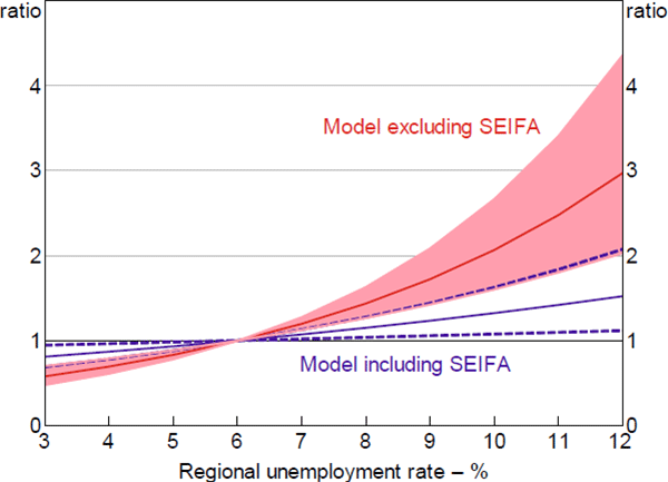
Notes: Hazard ratio set to 1 at the median value of x variable; shaded area/dashed lines denote 95% confidence intervals
Sources: ABS; Author's calculations; CoreLogic data; RBA; Securitisation System
The socio-economic profile of a region may be correlated with borrowers' probability of experiencing an ability-to-pay shock, and the severity of the shock, to the extent that it is correlated with unobserved borrower characteristics such as age, security of employment, financial literacy and understanding of the legal system. For example, Mincer (1991) finds that younger and less educated workers tend to suffer larger and more persistent employment loss during recessions – the effect of which may not be fully captured in the regional unemployment rate. Lower financial literacy may also be correlated with the presence of consumer debts, such as credit cards, that may lower borrowers' ability-to-pay threshold (Disney and Gathergood 2013). Holding all other covariates (including the regional unemployment rate) constant, loans located in postcodes with the highest socio-economic indices (SEIFA) were around 40 per cent less likely to enter arrears than those located in regions with low SEIFA (Figure 8).[21]
The share of regional employment in the mining industry is also strongly correlated with entries to arrears, even after controlling for regional unemployment rates. This may be related to reductions in income or lower job security beyond that indicated by regional unemployment rates, although we cannot rule out the possibility that mining regions may differ systematically in some other respect (see Section 7.2 for a discussion). Loans located in regions with the highest mining shares of employment were estimated to be twice as likely to enter arrears as those in regions with fewer jobs in the mining industry (Figure 9).
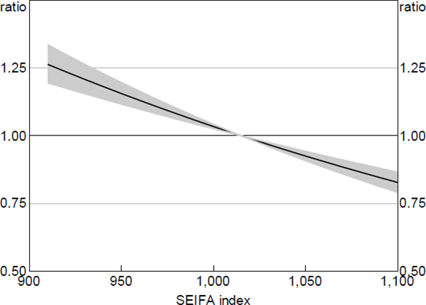
Notes: Hazard ratio set to 1 at the median value of x variable; shaded area denotes 95% confidence intervals
Sources: ABS; Author's calculations; CoreLogic data; RBA; Securitisation System
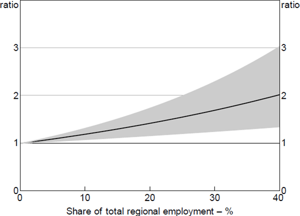
Notes: Hazard ratio set to 1 at the median value of x variable; shaded area denotes 95% confidence intervals
Sources: ABS; Author's calculations; CoreLogic data; RBA; Securitisation System
Borrower characteristics that are likely to be correlated with variability in income – and the probability of facing an ability-to-pay shock – were also positively correlated with the probability of entering arrears. Self-employed borrowers were estimated to be 19 per cent more likely to enter 90+ day arrears, consistent with these borrowers sometimes having less stable sources of income compared to employees. By contrast, mortgages backed by multiple borrowers were 27 per cent less likely to enter arrears; it is unlikely that all borrowers simultaneously experience an income reduction.
Increases in required loan repayments may cause liquidity-constrained borrowers to enter arrears, even without notable changes to their earnings. The magnitude of their effect on a borrower's ability to pay, however, would generally be less than that of the typical unemployment spell. Increases in required loan repayments are the only reduction to borrowers' ability to pay that we can directly observe in the data.
There have been two notable sources of increases to required repayments for borrowers over the sample period. First, lenders raised their standard variable rates for investor and interest-only (IO) loans in 2015 and 2017, typically by between 20 and 100 basis points (Kent 2017; Kohler 2017).[22] Second, a growing share of IO loans have had their IO periods expire over recent years, resulting in a step-up in total required payments by around 30 to 40 per cent for those loans (Kent 2018). To capture these effects, two variables have been included in the model: lagged changes in interest rates, expressed in buckets, and an IO period expiry indicator variable.
The model estimates suggest that an increase in interest rates in excess of 25 basis points was associated with a 19 per cent increase in the hazard of loans entering 90+ day arrears, relative to loans whose interest rate was unchanged. Most borrowers facing IO period expiries were able to transition to higher repayments without encountering repayment difficulties. Notwithstanding this, estimates suggest that borrowers whose IO period had expired in the previous six months were twice as likely to enter arrears compared to other loans paying principal and interest. However, this coefficient is likely to be upwardly biased due to selection bias – loans facing an IO period expiry may be riskier on dimensions other than those captured in the model.[23]
6.1.1.2 Ability-to-pay thresholds
Under the double-trigger hypothesis, various factors may influence the ability-to-pay threshold, that is, the size of the ability-to-pay shock that a borrower is able to tolerate before entering arrears. These include buffers that borrowers have built up through their loan repayments and savings, as well as the ratio of their loan repayments to income.
Borrowers who are ahead of their loan repayments may draw down upon their prepayment buffers in the event of an ability-to-pay shock, extending the time until they are behind on their repayment schedules. This may allow a borrower to avoid arrears, effectively raising the ability-to-pay threshold. The median borrower in the sample had a maximum of between one and six months of buffers at some point in time. Relative to the median borrower, borrowers who have ever had a buffer of over six months were 67 per cent less likely to enter 90+ day arrears, while a borrower who has never had a buffer greater than one month was 2.3 times more likely to enter arrears.
Likewise, loan serviceability affects the ability-to-pay threshold – borrowers facing a mild income shock may be able to continue making repayments if they have a low DSR, but are increasingly unlikely to be able to do so for higher DSRs. Model estimates suggest that this effect is important, with loans with high DSRs being around three times as likely to enter arrears as loans with low DSRs (Figure 10).[24],[25]
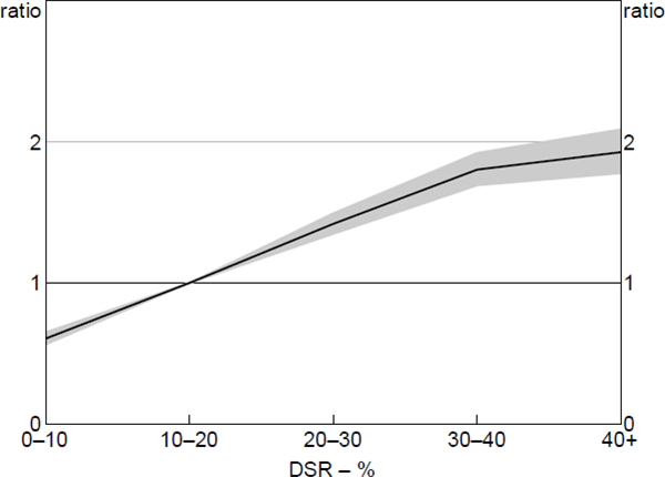
Notes: Hazard ratio set to 1 at the median value of x variable; shaded area denotes 95% confidence intervals
Sources: ABS; Author's calculations; CoreLogic data; RBA; Securitisation System
6.1.2 Equity
As highlighted in Hypothesis B, the double-trigger hypothesis implies no direct link between equity and entries to arrears. However, the probability of entering arrears may be weakly increasing in negative equity if borrowers' willingness to repay threshold is a function of equity. Empirical research by Gerardi et al (2018) suggests that borrowers facing an ability-to-pay shock may attempt to avoid arrears, and ultimately foreclosure, by cutting back on consumption expenditure if they have positive equity.[26]
The model estimates of the magnitude of the relationship between negative equity and entries to 90+ day arrears are surprisingly large; a loan that is deeply in negative equity was three times as likely to enter arrears as a loan with the median indexed LVR (Figure 11). The buckets specification is flexible enough to highlight nonlinearities. The probability of entering arrears increases gradually for loans with LVRs above 50, but does not accelerate for loans with negative equity. It is possible that this result may reflect a correlation with ability-to-pay factors that have not been fully controlled for, such as changes in borrower income. This means that the equity result is inconclusive; it is not sufficient to refute the double-trigger hypothesis, but it also does not rule out the possibility that some borrowers with negative equity may strategically default.
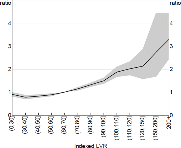
Notes: Hazard ratio set to 1 at the median value of x variable; shaded area denotes 95% confidence intervals
Sources: ABS; Author's calculations; CoreLogic data; RBA; Securitisation System
The above ability-to-pay results confirm Hypothesis A, whereas the surprisingly large hazard ratios for equity prevent me from confirming Hypothesis B. That said, there may be unobserved ability-to-pay factors that are correlated with equity, and the ability-to-pay hazard ratios are larger than the equity hazard ratios. Therefore, the first stage results are broadly consistent with the double-trigger hypothesis.
6.2 Second-stage Hazard Model: Transitions from Arrears
6.2.1 Equity and housing market turnover
The double-trigger hypothesis predicts that the degree of negative equity is the main determinant of whether a loan in arrears transitions to foreclosure. Consistent with Hypothesis C, model estimates suggest that the probability of loans transitioning into foreclosure is increasing in the degree of negative equity. Meanwhile, the probability of loans curing or fully repaying declines for loans with negative equity. Loans that are deeply in negative equity (at the point of entering arrears) are around five to eight times as likely to transition to foreclosure as a loan with the median LVR (Figure 12). The magnitudes of these hazard ratios are larger than in the first stage results. There are no distinct thresholds around which loans transition to foreclosure, in line with international evidence that suggests that borrowers have heterogeneous foreclosure costs and housing price expectations (Guiso et al 2013; Bhutta et al 2017).
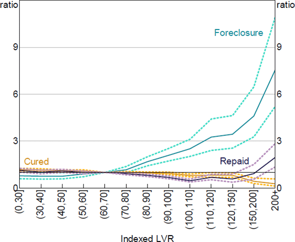
Notes: Hazard ratio set to 1 at the median value of x variable; dashed lines denote 95% confidence intervals
Sources: ABS; Author's calculations; CoreLogic data; RBA; Securitisation System
Although low turnover in a region may be symptomatic of other problems in that region, low turnover itself may also affect whether a borrower is able to avoid foreclosure by selling the property themselves. There are several channels through which this may occur, including by hampering price discovery, slowing sale times, increasing housing price variance (thereby increasing the probability that a loan has negative equity), and sending a negative signal to potential buyers (e.g. about the quality of properties on the market). Even after controlling for region remoteness and indexed LVRs, loans located in areas with lower turnover ratios (which were often regional areas) were around 40 per cent more likely to transition to foreclosure than those in areas with high turnover ratios (Figure 13). They were also less likely to be fully repaid. These results suggest that nonlinearities may be a risk in a housing market stress scenario, where low housing turnover may exacerbate foreclosures.
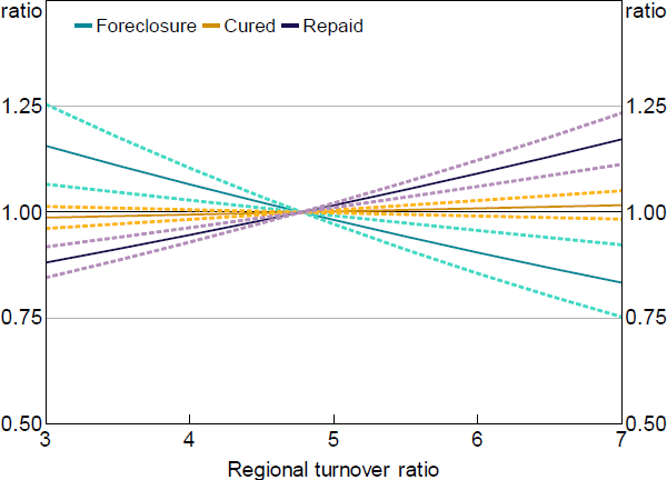
Notes: Hazard ratio set to 1 at the median value of x variable; dashed lines denote 95% confidence intervals
Sources: ABS; Author's calculations; CoreLogic data; RBA; Securitisation System
In addition to these effects, loans in regional towns and remote areas were around 50 per cent more likely to proceed to foreclosure than their counterparts in larger cities (all else equal), and were less likely to fully repay. This might be due to nonlinearities in housing market conditions, such as borrowers having lower housing price growth expectations or through longer sale times not being fully accounted for by the housing turnover ratio. Alternatively, it may reflect slower recovery times from ability-to-pay shocks in regional areas due to shallower labour markets.
6.2.2 Ability-to-pay factors
The hazard ratios for ability-to-pay factors in the second-stage model for foreclosures were not statistically significant and were small in magnitude, with the exception of the regional unemployment rate (Figure 14). These results are consistent with the double-trigger hypothesis and in line with Hypothesis D, that is, the size of the ability-to-pay shock is not relevant for transitions to foreclosures, but a reversal of the shock (e.g. the borrower regaining employment) may allow the borrower to cure.
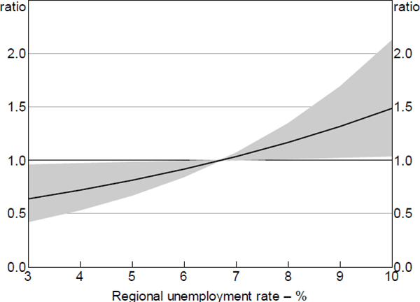
Notes: Model excluding the SEIFA variable; hazard ratio set to 1 at the median value of x variable; shaded area denotes 95% confidence intervals
Sources: ABS; Author's calculations; CoreLogic data; RBA; Securitisation System
International evidence suggests that a higher unemployment rate impairs a borrower's ability to cure by regaining employment. For example, Adelino et al (2013) point to the rise in the unemployment rate as a factor in the reduction in cure rates in the United States from around 70 per cent to 25 per cent between 2006 and 2009. However, the hazard ratio estimated in my model for loan cures was relatively small in magnitude; the regional unemployment rate being a poor proxy for individual unemployment may again make it difficult to estimate the true effect of unemployment.
6.2.3 Recourse
It is likely that full recourse to borrowers' other assets is a significant deterrent to foreclosure in Australia, however, its effect is difficult to measure in the absence of data on borrowers' other assets and debts. In jurisdictions with full recourse, borrowers' total equity position should be measured by their total debt-to-assets ratio, rather than indexed LVR. While this information is not available in the Securitisation Dataset (or in most loan-level datasets used in international studies), several variables may be partial proxies.
Investors and borrowers with high incomes may be likely candidates to have other assets that may have positive net worth and therefore reduce the borrowers' probability of foreclosure for a given indexed LVR. The results do not support this hypothesis. The hazard ratio for the high income dummy is not statistically significant in the second-stage model. Further, while investors were less likely to enter arrears in the first-stage model, having entered arrears, they were more likely to proceed to foreclosure in the second-stage model.[27] A number of competing factors may explain this result. For example, Albanesi, De Giorgi and Nosal (2017) argue that investors may be more likely to take on more risks or be more strategic in their decision-making due to a lack of sentimental attachment to the property or moving costs.
6.2.4 Restructuring arrangements
An important control in the second-stage model is whether the borrower had obtained any restructuring arrangements (including through hardship provisions), which are designed to assist the borrower with curing. Restructuring arrangements reduced the hazard of foreclosure by 60 per cent for the full subset of loans, and by 40 per cent for loans with negative equity. As well as increasing the likelihood of a loan in 90+ day arrears curing, restructuring arrangements also extend the time that loans spend in arrears.
Footnotes
Appendix B also includes results for the competing risks, as well as models estimated over the subset of loans with negative equity and the subset of loans located in mining-exposed regions. Multinomial logit results, as a robustness check, can be found in Appendix C and are also broadly consistent with the results presented below. [17]
Models that include only the main variables of interest have concordance ratios around 0.75. Concordance ratios are approximately equal to the area under the ROC curve for Cox models. [18]
In general, multicollinearity should not be dealt with by excluding relevant variables (due to omitted variable bias). But I am using these variables as proxies for an ability-to-pay shock. So omitting the socio-economic index is fine as long as the regional unemployment rate effect is interpreted as a combination of the true effect and any correlated changes in the socio-economic index. [19]
This hazard ratio is from the model estimated without the socio-economic index. In the model with the socio-economic index, the regional unemployment hazard ratio is 1.08. [20]
The Socio-Economic Indexes for Areas (SEIFA) are constructed by the Australian Bureau of Statistics from Census indicators such as unemployment, educational attainment, English language proficiency and car ownership. I use the socio-economic indices of relative advantage and disadvantage, which are at the postcode level (a finer level of aggregation than other regional statistics used throughout this paper). [21]
This was largely in response to regulatory measures introduced by the Australian Prudential Regulation Authority on the share of lending to investors and for IO loans. [22]
In particular, many astute IO borrowers who were not liquidity constrained had already voluntarily switched to making principal repayments to avoid the increase in interest rates on IO loans (see also RBA (2018)). [23]
The magnitude of the DSR estimates is larger than is typically found in the international literature. [24]
Surprisingly, borrowers that had high incomes (defined as a combined indexed income above $180,000) were more likely to enter arrears, all else equal. [25]
Another possibility is that negative equity may reduce a borrower's ability to avoid arrears through full repayment, either by preventing a borrower with an unaffordable loan from refinancing or because the borrower may be reluctant to sell the property due to loss aversion. This is an example of the competing risk not being independent of the event of interest; negative equity reduces the probability of the borrower experiencing the competing risk and therefore indirectly increases the probability of experiencing the event of interest. The Cox model assumes that competing risks are independent and does not capture the increase in risk implied in this example. [26]
These results also hold when the model is estimated over the subset of loans with negative equity. [27]