Research Discussion Paper – RDP 2018-04 DSGE Reno: Adding a Housing Block to a Small Open Economy Model
1. Introduction
Economic activity in the Australian housing market has increased substantially over the past five years, attracting considerable interest from academics and policymakers.[1] Housing investment, for example, has grown by about 30 per cent since the end of 2012 (Figure 1). The expansion in housing investment has helped to partially offset the large decline in mining investment associated with the downswing in the recent commodity price cycle. More generally, the housing market has played an important role in the transition of the economy away from the mining boom (e.g. Lowe 2015).
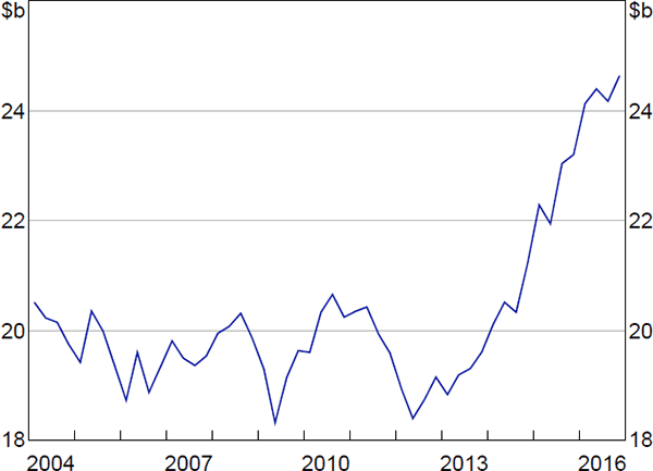
Sources: ABS; RBA
Against this background, the goal of this paper is to explicitly capture housing investment dynamics within a multi-sector model that is fit to the Australian economy. It is important to explicitly account for the housing sector, as there are many economic reasons to think that the housing sector, and in particular housing investment, may behave differently than other non-tradeable goods and services sectors. For example, Lawson and Rees (2008) find that investment in housing plays a particularly significant role in the transmission of monetary policy in Australia.
Moreover, research on housing and the macroeconomy shows that movements in housing markets are not just the consequence of wider macroeconomic developments, but can also be important impulses to business cycle fluctuations. Iacoviello and Neri (2010), for example, study housing in a multi-sector estimated dynamic stochastic general equilibrium (DSGE) model and conclude that shocks emanating from the housing market have noticeable effects on the real economy, especially on consumption. Muellbauer (2015) cites evidence from several model-based and econometric studies to argue that housing is a significant determinant of inflation in the United States.
Our starting point is the model in Rees, Smith and Hall ((2016); henceforth RSH). The RSH model is a multi-sector DSGE model designed from the ground up to explain aggregate variables that are relevant to the Australian economy and to capture the relative importance of, and interaction between, different sectors within a small open economy setting. It complements the Reserve Bank of Australia's suite of economic models, and has been in use for a few years as an analytical tool to conduct scenario analysis. We leave the key features of the RSH model intact, but incorporate a standalone housing sector into the existing framework.
To do this, we propose a general and straightforward modelling approach that may be applied to a wide variety of existing DSGE models. The approach generates a number of intuitive predictions, such as an increased sensitivity of housing investment to monetary policy, but leaves the aggregate predictions of the original model broadly unchanged. Specifically, we modify the RSH model along two dimensions. On the production side, we split the non-tradeable sector into a housing services sector and a non-tradeable excluding housing sector. On the demand side, we assume that households gain additional utility by holding housing stock. Therefore, in our framework, the housing stock is used by the housing services sector, along with other inputs, to produce housing services that form part of agents' consumption bundle. In addition, the housing stock also enters agents' utility function directly, separate from consumption.
The separation of the consumption of housing services from investment in the housing stock has a number of advantages. First, it allows for greater consistency between key macroeconomic variables such as GDP and CPI inflation, both of which have a large weight placed on housing services, and their model counterparts.[2],[3] This consistency is particularly important in our application as the model is primarily used for scenario analysis (examining the implications of different scenarios for key macroeconomic variables), and so we want the dynamics and definitions of the model variables to be as similar as possible to those of their real-world counterparts.
The second advantage of the separation is that it allows us to differentiate changes in the level of the housing stock that are driven by changes in the supply of and demand for the stock, from those driven by changes in the productivity of the housing stock in producing housing services. In turn, this also allows us to consider a broader range of scenarios, including: changes in the demand for the housing stock due to changes in tax treatments, which influence the post-tax return on housing and therefore households' willingness to hold housing assets; and increases in the productivity of the housing stock due to increased density of the housing stock, which would imply that, for a given amount of housing investment and capital, more housing services could be generated. The latter scenario is particularly interesting in the context of Australia, where the recent expansion of housing investment has been concentrated in the high density segment of the market.
Our preference assumption has implications for both the steady-state and dynamic properties of the model. First, because households gain utility from holding housing stock, they require a lower rate of return in steady state compared to the case of no housing stock in the utility function. This implies a higher level of housing stock in steady state, which is a key feature of the data. Indeed, without the assumption that the housing stock appears in the utility function, our model has difficulty matching the relative proportion of housing held by households in the data. Second, housing investment is more responsive to changes in the real interest rate compared to the case without housing in the utility function, which is consistent with empirical evidence on the relatively high sensitivity of housing investment to changes in interest rates (e.g. Lawson and Rees 2008). Finally, including the housing stock in the utility function also generates a positive correlation between real housing wealth (measured by the housing stock) and consumption. This is qualitatively similar to the housing wealth effects documented empirically in Australia by Dvornak and Kohler (2007) and Gillitzer and Wang (2015), and to the effect of the collateral constraints included in Iacoviello (2005) and Iacoviello and Neri (2010).
There are a number of justifications for treating the housing stock differently from other forms of capital and including it directly in the utility function as well as assuming that it is an input into housing services. One justification is the empirical observation that households tend to treat housing differently to other assets. Home ownership – in Australia and in many other developed countries – makes up a significant proportion of household wealth, and it is well-known that households' decisions with respect to their housing wealth often differ from the standard predictions of models of consumption and saving. For example, households typically dissave their housing wealth in retirement at rates below what the classical life-cycle model would predict, which Skinner (1996) argues could reflect the use of housing wealth as a form of self-insurance. Meanwhile, Nakajima and Telyukova (2013) use cross-country data and find that households tend to not use their housing wealth to respond to income shocks in the same way as they do other assets, which suggests that housing is not accumulated for precautionary savings motives in order to smooth consumption in the same way as other assets.
Another justification for including the housing stock in the utility function is the differential tax treatment of housing assets in Australia. In Australia, landlords can deduct expenses related to investment properties from their gross income, whereas expenses incurred in operating a business are generally quarantined to business income.[4] Meanwhile, owner-occupier housing receives preferential capital gains tax and pension assets test treatment, relative to other assets. Since we do not model a detailed fiscal sector, including the housing stock in the utility function acts as a proxy for these taxation features by providing households with an extra incentive to invest in and accumulate housing.[5]
Compared to the existing literature on the modelling of housing, our approach shares some similarities with Iacoviello-type models, which are used extensively in the literature (e.g. Iacoviello 2005; Iacoviello and Neri 2010). In these models, the housing stock also enters agents' utility function directly. However, it enters as a second consumption good to reflect housing services, which are assumed to be directly proportional to the housing stock. In our model, the housing stock is used to produce housing services, which are incorporated into the consumption bundle, but it also provides utility directly. Therefore, while preferences have a similar functional form in Iacoviello-type models, the interpretation is slightly different in our approach.
The other main difference is that in Iacoviello-type models housing serves as collateral for loans, whereas we abstract from debt dynamics implied by liquidity constrained households, instead focusing on housing investment decisions. We do so to maintain the standard representative agent framework and keep our model consistent with RSH. Although this simplification prevents us from incorporating collateral effects – likely to be important in trying to satisfactorily model the price of the existing housing stock, which is the price of interest for the housing sector in Iacoviello-type models – we show that our model does a good job in capturing aggregate and housing sector dynamics. Therefore, our specification represents a parsimonious, but still effective way to capture housing investment dynamics within a multi-sector model.[6]
We estimate the model using standard Bayesian techniques. We test its out-of-sample forecast accuracy using a pseudo forecasting experiment. We find that the model has reasonable out-of-sample forecast properties, especially for housing investment and value-added growth. While the model is not intended to be used for forecasting, its reasonable forecast performance provides evidence that it adequately captures relevant economic dynamics.
We also compare the impulse response functions of our model to those arising from RSH and from structural vector autoregression (SVAR) models for monetary policy shocks. Relative to RSH, the introduction of the housing sector increases the persistence of the output response to monetary policy shocks, while the magnitude of the response of inflation is relatively unchanged. These results are consistent with evidence arising from SVAR models estimated with the same disaggregated data.
We then explore the model dynamics associated with the different shocks in the housing sector. We show that shocks to the housing services sector have quite different effects on the economy than shocks that affect the stock of housing directly. In particular, negative shocks to the productivity of housing services tend to be inflationary, whereas negative shocks to the housing stock (housing preference or investment shocks) tend to be deflationary.
Finally, we use the model to assess the contribution of the housing sector to aggregate GDP growth and CPI inflation since the end of the mining boom in 2012. We find that housing investment played a significant role in driving growth and inflation over the past five years, adding a ½ percentage point to GDP growth and a ¼ percentage point to inflation, both in year-ended terms. We also find that the significant increase in housing investment has been primarily driven by the endogenous response of monetary policy to negative commodity price movements. In other words, monetary policy has largely been implemented as one would have expected based on past policy decisions and the fall in output and inflation observed during this period. Meanwhile, shocks emanating from the housing sector have actually weighed on housing investment, which means that housing investment has been lower than what the model would have predicted given the macroeconomic environment. This could reflect, for instance, capacity constraints in the sector or even the effect of changes in lending standards in recent years.
2. The Model
In this section, we provide a brief overview of the structure of the multi-sector model. We then present the household decision problem, an overview of the different sectors of the economy, and a brief discussion of the world economy model. We explain the accounting identities and the aggregation of the various sectors into the economy-wide aggregates. To build intuition for the economics behind the utility function specification, we also explore the steady-state properties of the housing sector using some partial-equilibrium comparative statics.
2.1 Overview
The multi-sector model we propose is a standard small open economy, sticky price, DSGE model. It represents an extension of the main DSGE model used by the Reserve Bank of Australia for policy analysis. The structure of the economy and the flows of real goods and services are shown in Figure 2.
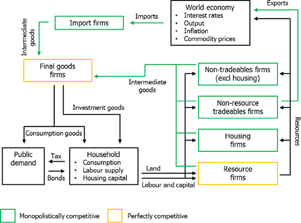
The small open economy – Australia – consists of households and firms that produce and consume in six distinct sectors. There are five intermediate goods and services-producing sectors: resource (mining), non-resource tradeable (manufacturing and agriculture), non-tradeable excluding housing, housing, and imported goods and services. The resource sector is modelled as perfectly competitive and takes the world price of the resource good as given. The remaining sectors are monopolistically competitive and have some power to choose the prices of the goods they sell. Price changes for monopolistically competitive firms are subject to Rotemberg (1982) style price adjustment costs. Wages in all domestic production sectors face similar adjustment costs. These adjustment costs generate price and wage stickiness in the model. Intermediate goods and services, produced domestically and imported from abroad, are combined into final goods by the perfectly competitive final goods sector, which provides goods for household and government consumption as well as business investment.
Households derive utility from consumption of the composite final good and from the level of the housing stock in the economy, and derive disutility from labour supplied to firms in the four domestic intermediate production sectors. Households earn wages from labour supplied, rents from their ownership of capital, and dividends from ownership of firms. Households may also purchase domestic and foreign nominal bonds.
Monetary policy in the model follows a Taylor-type rule that responds more than one-for-one to changes in inflation and positively to changes in real GDP growth. Fiscal policy is assumed passive with lump-sum taxation.
The world economy is significantly less detailed. The world is modelled as a two sector closed economy version of the model just described, and also features price stickiness. It purchases resources and tradeable goods from Australia, and sells tradeable goods to Australia. Households in the world economy may invest in their own and Australian nominal bonds.
2.2 The Household's Decision
The household's decision problem is to choose consumption, hours worked, and the level of the housing stock to maximise expected utility subject to a budget constraint. In particular, the household consumes a composite consumption good that is a constant elasticity of substitution (CES) aggregate of all intermediate goods, including housing services. In addition, the households also gain utility directly from the level of the housing stock in the economy. Therefore, housing-related quantities enter the utility function in two different ways. This specification provides us with a demand for housing services and a separate supply of housing stock. One can think of this as separating the household's need to consume housing services from their preference for home ownership. These two quantities, in principle, can move somewhat independently of one another.
Formally, we assume that there is a continuum of identical households indexed by i and distributed uniformly on the unit interval. The households choose a sequence of consumption, C(i)t, hours worked, H(i)t, and housing capital stock, K(i)d,t, to maximise the following utility function:
subject to the following budget constraint:
Households' preferences are subject to three autoregressive preference shocks ζC,t,  and ζH,t and exhibit habit persistence in both the level of consumption, b, and the level of the housing stock, bd. Ad and AH are normalising constants that pin down the steady state of the model so that it matches the data. Total hours worked Ht is an index composed of the hours allocated by households to each different production sector:
In the budget constraint, h(i)j,t and W(i)j,t denote hours worked and the nominal wage of household i in sector j; hj,t and Wj,t are average hours and wages in sector j, respectively;  is the wage adjustment cost in sector j; I(i)j,t and K(i)j,t are investment and capital, respectively, by household i in sector j; L is land; Δ(i)t and T(i)t are dividends and lump-sum taxes, respectively; Pt is the price level; St is the nominal exchange rate; ψt is a risk premium shock; B(i)t is the amount household i has invested in one-period risk-free nominal bonds; Rt is the nominal interest rate factor, and starred variables denote foreign quantities. The four domestic production sectors of the economy are denoted j = {n, m, z, d}, where n is non-tradeable excluding housing, m is non-resource tradeable, z is resources, and d is the housing (dwelling) sector.[7]
The final term of the budget constraint captures Rotemberg (1982) style wage adjustment costs with indexation, which we use to introduce wage stickiness into the model. The specification follows Burgess et al (2013). We assume that workers have heterogeneous skills. Firms purchase a bundle of labour from households that includes workers of all types:
Workers, therefore, have some bargaining power over their wages and take into consideration overall demand for labour and average wages in the market when negotiating. In addition, wage changes may be indexed to a combination of previous period's sectoral wage growth Πw,j,t − 1, and steady-state sectoral wage growth Πw,j,ss. The parameter  determines the degree of substitutability among differentiated labour inputs in sector j.
Households are homogenous, so individual consumption and saving decisions mirror the aggregated decisions. The aggregate capital stock of each sector in the economy evolves according to the following law of motion:
where δj is the depreciation rate of capital in sector j ∈ {n, m, z, d}, Ft (·) is the capital adjustment cost, and ϒt is an autoregressive investment adjustment cost shock.[8]
2.3 Sectoral Production
There are three monopolistically competitive intermediate goods-producing sectors in the model, which all share the same underlying structure: the non-tradeable excluding housing, the non-resource tradeable and the housing sectors. Additionally, there is a monopolistically competitive intermediate import sector and a perfectly competitive resource sector. The perfectly competitive final goods sector assembles the domestically sold output of these five sectors.
2.3.1 Intermediate monopolistically competitive goods and services producers
In the three monopolistically competitive producing sectors, we assume that there is a continuum of firms, indexed by k, that produce different intermediate goods using three factors: capital, labour, and the resource good. The firms sell their output to a wholesaler, who combines the differentiated intermediate goods into a homogenous good for sale in the final goods and services sector using a CES production technology:
where Y(k)j,t is output of firm k, and  governs the degree of substitutability among the different intermediate goods in sector j. The demand for each firm's output is given by:
Given the demand for a firm's product, the firm must choose the amount of capital and labour to hire, the price of their product, and the amount of resources to use in production. These decisions are mostly the same across the three intermediate domestic goods-producing sectors except for the tradeable sector, where firms additionally must choose how much to export and at what price. The decision in this case, though, mirrors the decision for the domestic market. Therefore, in the interest of space, we present only the decision problem for firms selling in the domestic market.[9]
Each intermediate firm produces a unique variety of goods and services using the following production function:
where h(k)j,t, K(k)j,t, and Z(k)j,t are the quantities of each input used by the kth firm, aj,t is a sector-specific autoregressive technology shock in sector j, αj and γj are the labour and capital shares, respectively, in sector j, and Mt is an aggregate permanent labour-augmenting technology shock that follows a process made up of two components: a random walk with drift component and an autoregressive component.[10] A firm's objective is to choose a sequence of factor inputs and prices to maximise the expected discounted value of profits into the infinite future, subject to demand for Y(k)j,t, where a firm's real profit in period t is given by:
The firm's pricing decision is subject to a quadratic price adjustment cost, which is scaled by  .
.
In addition, firms may index their price to a combination of πj,t − 1 and Πj, which are the previous period's sector-specific inflation rate and the steady-state sectoral inflation rate, respectively.
The MC(k)j,t are the marginal costs for firm k in sector j, which take the form:
where  is a white noise mark-up shock that increases marginal costs in sector j, and Pz,t is the domestic currency price of commodities.
In the case of housing services production, the intermediate producer can be thought of as professional property developers and managers. These developer/managers rent housing stock from households and combine it with labour and resources inputs to produce housing services. The housing services are then sold to the final goods producers to be combined with all other intermediates, which in turn are sold on to households as part of the CES consumption bundle. The price for housing services, therefore, reflects a composite of rents, new dwelling prices and real estate services, which are the main housing components that are included in the CPI. As discussed in the introduction, this represents a fundamental difference compared to Iacoviello-type models, where the price of housing is a measure of the sale price of new and existing real estate.
2.3.2 Imports, resources and final goods sectors
2.3.2.1 Imports sector
Firms in the imports sector, f, import differentiated goods and services from overseas, which they sell to wholesalers as the other intermediate sectors do. The marginal cost of importing goods and services by firm k is given by:
where  is an autoregressive mark-up shock. The firms seek to maximise expected profits by choosing a sequence of prices and the amount of goods and services to import, subject to demand for Y(k)f,t and quadratic price adjustment costs. Real profits in the sector are thus given by:
2.3.2.2 Resource sector
The resource sector is perfectly competitive and produces a homogeneous resource good. The resource good production function is given by:
where the stationary sector-specific technology shock takes on the same functional form as in the other sectors. The resource firms take the price as given and choose capital and labour to maximise profit, which is given by:
Following RSH, we assume that the law of one price holds for resources in the long run. However, we allow for a delay in the short-term pass-through of global resource price movements to the domestic price. This assumption captures the fact that a fraction of the resources exported from Australia are priced using contracts, which are only revised periodically, and that firms often hedge their foreign currency exposures. Therefore, the domestic price is assumed to follow:
where  denotes the price in foreign currency terms, and St is the nominal exchange rate.
2.3.2.3 Finals goods sector
The final goods sector purchases the homogenous composite goods from the wholesalers and assembles them into final goods using the following production function:
where ωn + ωm + ωd + ωf = 1 and govern the shares of each sector's output in the final domestic good,  stands for tradeable goods sold domestically, and DFDt is domestic final demand. Profit maximisation by the final goods producers implies the following aggregate price index:
2.4 Fiscal and Monetary Policy
Following RSH, fiscal policy is assumed to be passive. The government issues bonds and raises lump-sum taxes for expenditures. The government's budget constraint is given by:
Public demand, Gt, is assumed exogenous and takes the following form:
where g determines public demand's steady-state share of GDP. The lump-sum taxes assumption implies that Ricardian equivalence holds in the model, meaning that the timing of taxation does not affect households' and firms' decisions. In addition, we assume that government debt is held in zero net supply.
Monetary policy is assumed to be active and follows a Taylor-type rule. Therefore, short-term nominal interest rates are set according to:
where πt is the CPI inflation rate,  is real GDP (value added measure), Qt is the real exchange rate, ρr governs the degree of interest rate smoothing, and εr,t is a monetary policy shock. The parameters R and Π are steady-state interest rates and inflation, respectively.
2.5 Market Clearing and the Current Account
The goods market clearing conditions are:
The first condition requires all tradeable goods and services produced to be sold domestically or abroad. The second condition requires all resource goods produced to be sold abroad or to the three intermediate production sectors. The third condition says that all final goods must be sold to consumers, the government or invested.
The net foreign asset position of the economy is given by the current account:
where NXt is nominal net exports. Net exports in this case are equal to the sum of the exported traded goods and the traded resources, less imports:
In addition, the non-tradeable, tradeable, and housing sectors all use resources as inputs. This introduces a wedge between the production and the value added in these sectors. Therefore, the relevant concept of GDP in this case requires a value-added computation. Following RSH, we do this calculation by subtracting out the value of the resource input in each intermediate sector using steady-state prices Pj. For example,  . Therefore, real GDP is defined as:
Finally, the following uncovered interest rate parity (UIP) condition holds in the log-linearised model:
2.6 The Foreign Economy
The foreign economy is modelled as a standard closed economy sticky-price model. The log-linearised equations of this model are given by:
where Equations (28) and (29) together form the IS relationship, Equation (30) is the Phillips curve, and Equation (31) is the monetary policy rule. The foreign demand shock,  , and the foreign mark-up shock,
  , are assumed to follow autoregressive processes, while the remaining shocks are assumed to be white noise.
Commodity prices are assumed to follow an exogenous autoregressive process, which depends on its own shock and on the foreign demand shock:
where  is the relative price of the resource good in terms of the foreign currency.
2.7 Understanding Housing Capital Stock in the Utility Function
Adding the housing stock to the utility function has implications for the steady-state and dynamic predictions of the model. To build intuition for these effects, we present some partial equilibrium analysis using the steady-state relationships. This analysis allows us to look at the supply and demand relationships for the housing stock implied by the model and to do some basic curve shifting exercises. The dynamic general equilibrium predictions of the model are discussed in Sections 4 and 5.
The addition of the housing stock to the utility function primarily affects the supply of housing in the housing capital factor market. The capital factor markets in the model are perfectly competitive and can be illustrated using supply and demand schedules. The suppliers of the housing stock in this economy are the households. Supplying housing is one way in which households can save, and the stock of housing generates utility for the households. The demand for the housing stock comes from the firms in the housing services sector. These firms combine the housing stock with labour and resource goods to produce housing services, which are sold to the final goods producers and eventually to households for consumption. Therefore, the households' supply of housing may be thought of as the proportion of their portfolios invested in residential real estate.
To understand the effect of our preference assumption, we first discuss the households' supply of capital to any sector j when capital is not included in the utility function. In this case, the steady-state supply of capital is a fixed share of household saving that is determined solely by its return.
The return is pinned down by aggregate productivity, the household's discount rate, and the depreciation rate:
where μ is the steady-state labour-augmenting productivity growth rate. This relationship implies that households are willing to supply whatever the amount of capital the market demands at the current returns, and therefore, it generates a perfectly elastic supply schedule (represented by the horizontal line in Figure 3). The demand for capital comes from the marginal productivity of capital implied by the production technology. The production technology is Cobb-Douglas in all sectors so there are diminishing returns to capital, which give rise to the standard downward sloping demand schedule (Figure 3).
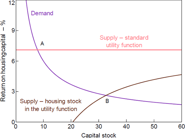
When we include the housing stock in the utility function, the household's supply schedule for housing capital is changed. Since households derive utility from holding the housing capital stock, they invest more in this sector. In doing so, they weigh the utility they get from the current and future level of the housing capital stock with the utility of consumption, which gives rise to the following supply schedule:
where λd,ss is the steady-state ‘shadow’ price of housing (i.e. the Lagrange multiplier associated with housing capital from the household's constrained optimisation problem), which is equivalent to the marginal utility of consumption.
Equation (34) implies an upward sloping relationship since gross steady-state productivity growth is assumed greater than one and habit persistence is less than one (Figure 3). Intuitively, the supply curve slopes upward because of the assumption of diminishing marginal utility of the capital stock in the preference specification. Households are no longer willing to supply whatever amount of capital is demanded because higher levels of capital stock mean lower marginal utility, and therefore a higher rate of return on the housing capital stock is now required to induce more capital supply.
Moreover, when housing is included in the utility function, the supply curve for the housing capital stock is shifted to the right, relative to the case without housing in the utility function.[11] This reflects the fact that households gain utility from holding the capital and therefore require lower returns in steady state. Consequently, the steady-state rate of return is lower, while the steady-state level of housing is higher (point B in Figure 3 instead of point A). This higher steady-state level of housing turns out to be a key feature of the model, which helps it to match the data.
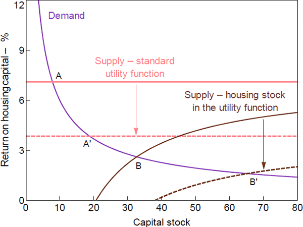
The differences in the supply curves, and their intersections with the demand curve, imply different responses of housing investment to changes in steady-state real interest rates. Figure 4 shows the predicted change in the capital stock for a decrease in the real interest rate due to an increase the household discount factor.[12] A fall in the steady-state real interest rate shifts the supply curve for the housing capital stock to the right. This shift results in a higher steady-state quantity of housing and pushes down the rate of return. Due to the different curvatures of the supply schedules, and the different initial conditions, the increase in housing is much larger in the case where the housing stock is included in the utility function, while the effect on the return is smaller (with the economy moving from point AꞋ to BꞋ in Figure 4 instead of from point A to B). Therefore, ceteris paribus, the same fall in interest rates generates a larger investment response when the housing stock is included in the household utility function, compared to the case when it is not included.
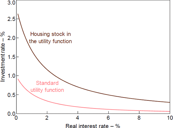
Figure 5 quantifies the difference in the investment response between the two cases for a range of steady-state values of the real interest rate. As the steady-state real interest rate falls, investment in the housing capital stock rises in both cases. However, the difference in the responses between the two cases increases as the interest rate approaches zero.
To summarise, in steady state, the assumption that the housing stock appears in the utility function implies that households hold more housing than would otherwise be the case, and that investment is more responsive to changes in the steady-state real interest rates. The increased sensitivity of housing investment to interest rates will carry over to the dynamic predictions of the model.
3. Estimation
We take the model to the data using a mix of calibration and estimation. As shown by Komunjer and Ng (2011), not all parameters of medium- and large-scale DSGE models are identified. Therefore, some parameters must be calibrated. We choose to calibrate parameters in the model that are known to be weakly identified in the literature and those which are most important for determining the steady state of the model. We calibrate these parameters to roughly match some key aggregate values, such as: the investment, consumption, import and export shares of GDP; and the housing share of the total capital stock. We estimate the remaining parameters, which mostly govern the dynamic predictions of the model, using standard Bayesian techniques. These include the exogenous shock processes, Phillips curve relationships, monetary policy parameters, and their counterparts in the world economy. Below, we provide a description of the data and the calibrated and estimated parameters.
We take a first-order approximation of the households' and firms' first-order conditions, and the capital accumulation equations around their respective steady states. We then use the software package Dynare to solve for the rational expectations solution of the model and to estimate parameters.
3.1 Data
We estimate the model using 26 macroeconomic data series. Of these, 22 series are Australia-specific, while the remaining ones capture movements in the world economy. The series and their sources are reported in Appendix A. To capture the housing sector, we consider four measures of activity: housing sector value added; the housing-related components of the CPI; a housing sector wage index; and housing investment. We use data from the March quarter of 1992 to the December quarter of 2016 for all series but the wage price indices, which are only available starting in the December quarter of 1997. We supplement these data with information on import volumes, public demand and capital stocks to calibrate the steady state of the model.
The world economy is summarised by major trading partner (MTP) GDP growth, the trade-weighted MTP inflation rate, the average interest rate in the G3 (United States, euro area, and Japan), and price growth in world commodity prices. The world economy is assumed to be exogenous to Australia and is estimated separately as in Kulish and Rees (2011). The Australian economy is summarised by standard aggregate variables such as GDP growth, consumption growth, CPI inflation and the cash rate, as well as several sector-specific growth and inflation measures.
3.2 Calibrated Parameters
Table 1 shows the values chosen for the calibrated parameters of the model. The key calibrated parameters are labour-augmented productivity growth, the discount factor, parameters of the various sector production functions, the elasticities of substitution between goods, and the consumption shares of the different sectors. These parameter choices follow RSH where possible. The production function parameters are chosen to reflect sectoral income shares observed in the data. We make some minor adjustments to the parameters to hit the steady-state targets.[13]
| Parameter | Description | Value |
|---|---|---|
| Technology and policy | ||
| μ | Steady-state labour-augmenting productivity growth | 1.008 |
| π | Steady-state inflation rate | 1.0062 |
| π* | Steady-state foreign inflation rate | 1.005 |
| ι | Risk premium scale parameter | 0.0001 |
| b* | Controls steady-state trade deficit | 0.25 |
| g | Controls share of public demand in GDP | 0.6487 |
| Households | ||
| β | Households' discount factor | 0.9996 |
| ωn | Controls share of non-tradeables in domestic final demand | 0.3970 |
| ωm | Controls share of non-resource tradeables in domestic final demand | 0.1118 |
| ωd | Controls share of housing in domestic final demand | 0.2447 |
| ωf | Controls share of imports in domestic final demand | 0.2465 |
| ζ | Intersectoral elasticity of substitution in domestic final demand | 0.8 |
| ξ | Elasticity of substitution between domestic and foreign goods overseas | 0.8 |
| η | Labour elasticity | 1 |
| σ | Intersectoral labour supply elasticity | 1 |
| AH | Normalising constant for labour in the utility function | 4.4177 |
| Ad | Normalising constant for capital in the utility function | 0.3 |
| Non-tradeable sector | ||
| αn | Labour share | 0.71 |
| γn | Capital share | 0.24 |
 |
Elasticity of substitution between differentiated goods | 6 |
 |
Elasticity of substitution between differentiated labour | 0.25 |
| δn | Depreciation rate | 0.0047 |
| Φn | Investment adjustment cost parameter | 20 |
| Non-resource tradeable sector | ||
| αm | Labour share | 0.62 |
| γm | Capital share | 0.32 |
 |
Elasticity of substitution between differentiated goods | 6 |
 |
Elasticity of substitution between differentiated labour | 0.25 |
| δm | Depreciation rate | 0.0075 |
| Φm | Investment adjustment cost parameter | 20 |
 |
Controls share of non-resource tradeables that are exported | 0.6541 |
| Resource sector | ||
| αz | Labour share | 0.2 |
| αL,z | Land share | 0.5 |
| δz | Depreciation rate | 0.007 |
| Φz | Investment adjustment cost parameter | 20 |
 |
Steady-state foreign-denominated resource price | 1 |
| Housing sector | ||
| αd | Labour share | 0.32 |
| γd | Capital share | 0.64 |
 |
Elasticity of substitution between differentiated goods | 6 |
 |
Elasticity of substitution between differentiated labour | 0.25 |
| δd | Depreciation rate | 0.0023 |
| Import sector | ||
| θf | Elasticity of substitution between differentiated goods | 6 |
Table 2 shows the steady-state targets and the model-implied values given the chosen parameters. The model matches the data reasonably well. It does a particularly good job of matching the housing-related quantities, especially the housing capital stock's average proportion of the overall capital stock. Therefore, we believe the parameterisation chosen is appropriate moving forward. To reiterate the role that our preference specification plays, if the assumption that the housing stock is in the utility function is removed, but the same calibration is used, the housing share of the capital stock falls by around 10 percentage points.
We also make one calibration choice based on the dynamic predictions of the model. We calibrate the sectoral investment adjustment costs for the non-tradeable, tradeable, and resource sectors. Investment adjustment costs play a significant role in determining the response of sectoral investment to a monetary policy shock. Because only aggregate investment and housing investment are observable, the investment responses in the remaining sectors are not well-identified. Therefore, we calibrate investment adjustment costs to be relatively large in these sectors so that the model predicts more muted responses. As we show in Section 4.2, this is consistent with evidence based on a VAR model.
| Variable | Average 1993–2016 | Model prediction |
|---|---|---|
| Expenditure as a share of GDP | ||
| Consumption | 56.9 | 55.8 |
| Private investment | 21.3 | 22.5 |
| Public demand | 22.7 | 22.5 |
| Production as a share of nominal GVA(a) | ||
| Non-tradeable | 47.5 | 46.2 |
| Tradeable | 25.3 | 24.2 |
| Resource | 12.3 | 11.6 |
| Housing | 15.7 | 18.0 |
| Trade | ||
| Import share of GDP | 20.6 | 20.6 |
| Export share of GDP | 19.5 | 19.6 |
| Resource share of export value | 43.4 | 37.2 |
| Investment as a share of total investment(a) | ||
| Non-tradeable | 29.8 | 33.4 |
| Tradeable | 23.0 | 23.8 |
| Resource | 17.1 | 15.1 |
| Housing | 30.0 | 27.6 |
| Capital stock | ||
| Housing share of capital stock | 37.6 | 34.1 |
|
Note: (a) Based on broad definition of resource sector discussed in Rayner and Bishop (2013) |
||
Finally, we include a number of calibrated reconciliation/measurement error terms. Because we use chain volume measures for GDP growth and for the growth in value added in each of the intermediate sectors, these components are additive in levels in the model but are not additive in the data. Similarly, we use trimmed mean CPI inflation, but headline measures of sectoral inflation. Therefore, to account for these and any other differences between the data and their model counterparts, we include a white noise measurement error term for each observable series, apart from: the nominal and real exchange rates; commodity prices; domestic interest rates; and foreign and domestic aggregate inflation and GDP.[14] The errors are calibrated to be 10 per cent of the observed variance in the variable. We do not impose any structure on the correlation of these reconciliation shocks with one another.[15]
3.3 Estimated Parameters
We estimate the model using Bayesian techniques. We choose informative prior distributions for each of the model parameters of interest and use the Metropolis-Hastings algorithm to take draws from the implied joint posterior distributions. We follow RSH and Kulish and Rees (2011) and estimate the model in two stages. First, we estimate the world economy's structural parameters separately. We then take these parameters as given in the second stage, when estimating the structural parameters of the small open economy and the parameters of the exogenous shock processes.[16] For estimation, we take 100,000 draws of the posterior distribution and discard the first 20,000. We run multiple chains and assess convergence using Brooks and Gelman (1998) method included in Dynare.[17]
Table 3 shows the estimated parameter values for the world economy obtained in the first stage of estimation. The parameter estimates are in line with those obtained in the existing literature for estimation on US data, such as An and Schorfheide (2007) or Smets and Wouters (2007). In particular, the Taylor-rule coefficients fall within standard ranges found in the literature, with monetary policy responding aggressively to deviations of inflation from target and a much smaller response to changes in real output growth. In addition, the world Phillips curve is estimated to be relatively flat and output shocks tend to be much larger than inflation shocks.
| Parameter | Prior distributions | Posterior distributions | ||||||
|---|---|---|---|---|---|---|---|---|
| Shape | Mean | Std dev | Mode | Mean | 5th percentile | 95th percentile | ||
 |
Beta | 0.50 | 0.15 | 0.94 | 0.94 | 0.91 | 0.97 | |
 |
Beta | 0.50 | 0.15 | 0.55 | 0.53 | 0.34 | 0.71 | |
 |
Beta | 0.75 | 0.10 | 0.83 | 0.82 | 0.77 | 0.87 | |
| ρμ | Beta | 0.40 | 0.20 | 0.30 | 0.33 | 0.05 | 0.61 | |
 |
Normal | 1.50 | 0.20 | 1.37 | 1.41 | 1.17 | 1.63 | |
 |
Normal | 0.13 | 0.05 | 0.23 | 0.23 | 0.15 | 0.30 | |
 |
Beta | 0.50 | 0.15 | 0.94 | 0.94 | 0.91 | 0.97 | |
| θzy | Normal | 0.00 | 0.20 | 0.12 | 0.12 | −0.19 | 0.46 | |
| χ* | Beta | 0.30 | 0.15 | 0.23 | 0.27 | 0.09 | 0.46 | |
| κ* | Gamma | 1.00 | 0.80 | 0.97 | 1.52 | 0.42 | 2.63 | |
| Standard deviations (× 100) | ||||||||
 |
Gamma | 0.50 | 0.40 | 6.22 | 6.31 | 5.59 | 7.04 | |
 |
Gamma | 0.50 | 0.40 | 0.97 | 1.00 | 0.73 | 1.30 | |
 |
Gamma | 0.50 | 0.40 | 0.08 | 0.08 | 0.06 | 0.10 | |
 |
Gamma | 0.50 | 0.40 | 0.06 | 0.06 | 0.05 | 0.08 | |
| σμ | Gamma | 0.50 | 0.40 | 0.06 | 0.13 | 0.01 | 0.24 | |
Tables 4 and 5 show the estimated parameter values for the Australian economy. The estimates of the monetary policy rule are similar to those for the world economy, and those from RSH. Australian monetary policy responds aggressively to deviations in inflation from target and less so to changes in real output. Consistent with RSH, there is no evidence that monetary policy responds to changes in the real exchange rate. There is evidence of habit persistence in both the consumption of goods and in the holding of housing. The persistence in consumption is much larger than that associated with the holding of the housing capital stock. In part, this reflects the prior we impose, which implies that households are more willing to adjust their holdings of the physical housing stock than their consumption of the services it provides. We have a low prior value in this case because we also assume capital adjustment costs, so households already face frictions in adjusting the capital stock.
As in RSH, rather than estimating the price adjustment costs, about which we have no strong prior beliefs, we directly estimate the slopes of the Phillips curves. Each slope is just a monotonic transformation of the adjustment cost parameters. Specifically:
for  .
.
We, however, use different priors to those used in RSH. We use priors based on micro evidence from Sutton (2017). The estimated slopes reveal much flatter Phillips curve relationships in the housing and non-tradeable sectors than in the non-resource tradeable sector, while the degree of indexation to lagged inflation in these two sectors is higher. In terms of the model, this is consistent with a higher cost to adjusting prices and a higher dependence on recent conditions in these two sectors. We apply the same estimation strategy to the wage Phillips curves, though we use uninformative priors. The slopes of the wage Phillips curves are roughly the same across the sectors and are relatively flat in all cases. The degree of indexation is also similar across industries, revealing no significant differences in wage setting across the intermediate industries.
Finally, the estimated shock processes all exhibit moderate to high persistence. This is due to the fact that DSGE models under rational expectations lack significant propagation mechanisms for shocks. Therefore, to explain the persistence observed in data, the shock processes must be highly persistent. There are also a few persistence parameters that appear not to be well-identified. For example, the data does not add much to the priors on the autoregressive coefficient on either the housing stock preference shock or the labour supply shock.
| Parameter | Prior distributions | Posterior distributions | ||||||
|---|---|---|---|---|---|---|---|---|
| Shape | Mean | Std dev | Mode | Mean | 5th percentile | 95th percentile | ||
| Habit persistence and investment adjustment costs | ||||||||
| b | Beta | 0.50 | 0.20 | 0.90 | 0.90 | 0.85 | 0.94 | |
| bd | Beta | 0.20 | 0.10 | 0.16 | 0.21 | 0.04 | 0.36 | |
| Φd | Normal | 3.00 | 1.50 | 3.74 | 4.03 | 2.71 | 5.42 | |
| Monetary policy and UIP | ||||||||
| ρr | Beta | 0.90 | 0.03 | 0.87 | 0.87 | 0.84 | 0.89 | |
| ϕπ | Normal | 1.50 | 0.10 | 1.54 | 1.55 | 1.40 | 1.70 | |
| ϕdy | Normal | 0.20 | 0.03 | 0.21 | 0.21 | 0.17 | 0.25 | |
| ϕq | Normal | 0.00 | 0.05 | 0.00 | −0.01 | −0.04 | 0.03 | |
| Θψ | Beta | 0.50 | 0.15 | 0.07 | 0.08 | 0.03 | 0.13 | |
| Price and wage Phillips curves | ||||||||
 |
Gamma | 8.00 | 2.00 | 2.93 | 3.54 | 1.94 | 5.08 | |
 |
Gamma | 10.00 | 2.50 | 9.16 | 9.30 | 5.50 | 12.95 | |
 |
Gamma | 10.00 | 2.50 | 4.74 | 5.26 | 3.19 | 7.35 | |
 |
Gamma | 1.00 | 0.30 | 0.12 | 0.15 | 0.09 | 0.22 | |
 |
Gamma | 10.00 | 2.50 | 2.03 | 2.21 | 1.46 | 2.99 | |
| χn | Beta | 0.30 | 0.15 | 0.29 | 0.30 | 0.11 | 0.47 | |
| χm | Beta | 0.30 | 0.15 | 0.17 | 0.21 | 0.04 | 0.37 | |
 |
Beta | 0.30 | 0.15 | 0.08 | 0.12 | 0.02 | 0.22 | |
| χd | Beta | 0.30 | 0.15 | 0.63 | 0.62 | 0.45 | 0.79 | |
| χf | Beta | 0.30 | 0.15 | 0.15 | 0.17 | 0.05 | 0.30 | |
 |
Gamma | 50 | 30 | 0.13 | 0.19 | 0.09 | 0.29 | |
 |
Gamma | 50 | 30 | 0.10 | 0.14 | 0.06 | 0.21 | |
 |
Gamma | 50 | 30 | 0.12 | 0.13 | 0.07 | 0.20 | |
 |
Gamma | 50 | 30 | 0.15 | 0.19 | 0.10 | 0.27 | |
 |
Beta | 0.30 | 0.15 | 0.12 | 0.16 | 0.02 | 0.29 | |
 |
Beta | 0.30 | 0.15 | 0.20 | 0.25 | 0.10 | 0.39 | |
 |
Beta | 0.30 | 0.15 | 0.26 | 0.29 | 0.11 | 0.47 | |
 |
Beta | 0.30 | 0.15 | 0.10 | 0.13 | 0.03 | 0.22 | |
| Shock persistence | ||||||||
| ρg | Beta | 0.50 | 0.20 | 0.75 | 0.66 | 0.38 | 0.91 | |
 |
Beta | 0.50 | 0.20 | 0.54 | 0.54 | 0.36 | 0.72 | |
 |
Beta | 0.50 | 0.20 | 0.93 | 0.91 | 0.86 | 0.96 | |
 |
Beta | 0.50 | 0.20 | 0.50 | 0.51 | 0.17 | 0.85 | |
| ρϒ | Beta | 0.50 | 0.20 | 0.67 | 0.63 | 0.51 | 0.75 | |
 |
Beta | 0.50 | 0.20 | 0.62 | 0.59 | 0.45 | 0.74 | |
| ρψ | Beta | 0.50 | 0.08 | 0.78 | 0.77 | 0.73 | 0.82 | |
 |
Beta | 0.50 | 0.20 | 0.75 | 0.72 | 0.63 | 0.83 | |
 |
Beta | 0.50 | 0.20 | 0.98 | 0.96 | 0.92 | 1.00 | |
 |
Beta | 0.50 | 0.20 | 0.93 | 0.91 | 0.85 | 0.97 | |
 |
Beta | 0.50 | 0.20 | 0.75 | 0.71 | 0.62 | 0.81 | |
| Parameter | Prior distributions | Posterior distributions | ||||||
|---|---|---|---|---|---|---|---|---|
| Shape | Mean | Std dev | Mode | Mean | 5th percentile | 95th percentile | ||
| Policy and preferences (× 100) | ||||||||
| σg | Gamma | 1.00 | 0.80 | 1.23 | 1.22 | 0.99 | 1.40 | |
 |
Gamma | 1.00 | 0.80 | 4.49 | 4.54 | 2.89 | 6.15 | |
 |
Gamma | 1.00 | 0.80 | 5.97 | 5.82 | 3.38 | 8.23 | |
 |
Gamma | 1.00 | 0.80 | 0.36 | 0.86 | 0.03 | 1.68 | |
| σr | Gamma | 0.15 | 0.10 | 0.11 | 0.11 | 0.10 | 0.13 | |
| σψ | Gamma | 0.50 | 0.40 | 0.92 | 0.99 | 0.75 | 1.23 | |
| Production (× 100) | ||||||||
| σϒ | Gamma | 2.00 | 1.50 | 24.01 | 26.18 | 19.71 | 31.80 | |
 |
Gamma | 2.00 | 1.50 | 7.31 | 8.23 | 4.79 | 11.59 | |
 |
Gamma | 1.00 | 0.80 | 1.42 | 1.43 | 1.23 | 1.61 | |
 |
Gamma | 1.00 | 0.80 | 0.57 | 0.67 | 0.41 | 0.93 | |
 |
Gamma | 1.00 | 0.80 | 1.85 | 1.88 | 1.65 | 2.13 | |
 |
Gamma | 1.00 | 0.80 | 3.76 | 3.78 | 3.26 | 4.31 | |
| Price and wage inflation (× 100) | ||||||||
 |
Gamma | 0.50 | 0.40 | 0.35 | 0.36 | 0.30 | 0.43 | |
 |
Gamma | 0.50 | 0.40 | 0.54 | 0.54 | 0.45 | 0.63 | |
 |
Gamma | 0.50 | 0.40 | 2.59 | 2.68 | 2.23 | 3.07 | |
 |
Gamma | 0.50 | 0.40 | 0.18 | 0.19 | 0.15 | 0.22 | |
 |
Gamma | 0.50 | 0.40 | 1.00 | 1.02 | 0.86 | 1.20 | |
 |
Gamma | 0.15 | 0.10 | 0.05 | 0.05 | 0.02 | 0.07 | |
 |
Gamma | 0.15 | 0.10 | 0.10 | 0.10 | 0.08 | 0.12 | |
 |
Gamma | 0.15 | 0.10 | 0.19 | 0.19 | 0.15 | 0.24 | |
 |
Gamma | 0.15 | 0.10 | 0.21 | 0.22 | 0.18 | 0.25 | |
3.4 Forecast Performance
In this section, we assess the out-of-sample forecasting performance of the model. The DSGE model is not designed for forecasting. However, its pseudo out-of-sample forecast performance can be used to assess the model's ability to capture sectoral dynamics, in particular those related to the housing sector. Put another way, we can use the forecast performance as a goodness of fit measure.
In our forecasting exercise, we produce out-of-sample forecasts for a number of variables for horizons of 1 to 10 quarters ahead. We use a recursive strategy, extending the sample by 1 quarter at a time before producing each set of forecasts. Our first set of forecasts use data up to June 2002, and our last set of forecasts use data up to June 2014. Forecasts are then compared to the actual outcomes, and the errors are used to calculate root mean squared forecast errors (RMSFE) for each variable at each horizon.
Rather than re-estimating the model parameters with each new observation, we only update the parameters after an additional year of data (equivalent to four observations) becomes available. In addition to reducing computational time, this reflects more accurately the frequency with which DSGE models are typically re-estimated at the Bank.
We compare the DSGE model's RMSFE to two simple benchmarks. The first is the standard deviation of the actual outcomes over the full sample. This is equivalent to comparing the DSGE model's RMSFE to that of an ‘informed’ model, which forecasts the variables to be equal to their full sample means. As the full sample mean is not available to the DSGE model when it produces its forecasts, this represents a relatively high bar.[18] The second benchmark is the RMSFE from a ‘naïve’ model. We use an autoregressive model of order one (AR1) for each variable. Again, this is a reasonably high bar as it is generally quite difficult to forecast more accurately than an AR1 model. All variables considered are quarterly growth rates.
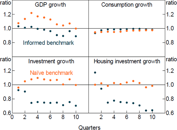
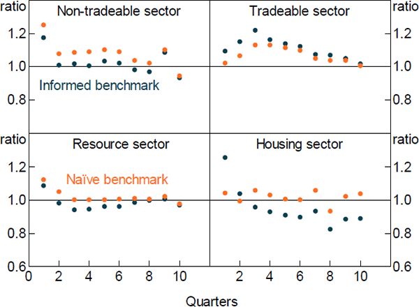
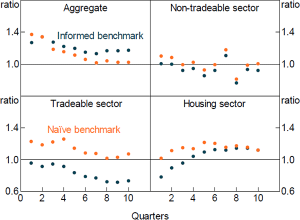
Figures 6 and 7 show the relative forecast performance of the DSGE model for GDP and its components. The DSGE model produces forecasts that are broadly comparable in terms of accuracy to those from an AR1 model at most forecast horizons, though its medium-term GDP forecasts are somewhat less accurate. It also performs favourably compared to the informed benchmark, particularly for housing sector value added, and housing and total investment. Figure 8 shows the relative forecast performance for inflation and its components. The DSGE model does not forecast aggregate inflation particularly well. This reflects the fact that it forecasts imported inflation poorly. In contrast, it does a reasonable job in forecasting the domestic components of inflation, particularly at longer horizons.
Overall, our model produces forecasts that are broadly comparable to both informed and naïve benchmarks. Its forecasts for housing sector variables are particularly good. This is reassuring, as it suggests that the DSGE model is adequately capturing housing sector dynamics, which is the intent of this paper.
Note: Ratio of DSGE model RMSFE to benchmark model RMSFE
Note: Ratio of DSGE model RMSFE to benchmark model RMSFE
Note: Ratio of DSGE model RMSFE to benchmark model RMSFE
4. The Transmission of Monetary Policy
This section compares the transmission of monetary policy in our model to RSH.[19] This allows us to quantify the differences in dynamics that come from the addition of the housing sector and the changes to household preferences. To this end, we use a modified version of RSH that includes our sticky wage specification, inflation indexation, and the same foreign sector as we consider in this paper.
4.1 Impulse Responses to a Monetary Policy Shock
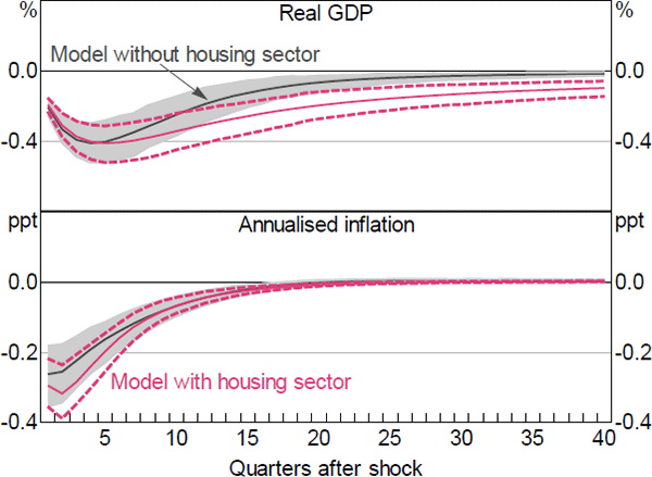
Figure 9 shows the responses of real GDP and inflation to a 100 basis point increase in the cash rate. Tighter monetary policy leads to a contraction in the real economy. GDP decreases by around 0.4 per cent at its peak, which occurs five quarters after the shock. The decline in GDP, which is within the range of estimates from empirical VAR models (e.g. Berkelmans 2005; Lawson and Rees 2008), is more persistent in our model than in RSH (the model without housing). This reflects more persistent declines in both consumption and investment. The increase in the cash rate lowers inflation slightly more than in the RSH model.
Note: 100 basis point increase in cash rate
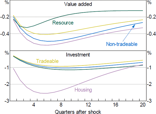
Figure 10 shows the responses of sectoral investment and value added in our model. These provide some insight into the model dynamics. Consistent with SVAR evidence we present below, the housing sector is the most interest-sensitive sector – particularly housing investment, which declines by around 2.5 per cent, similar to Lawson and Rees (2008). Meanwhile, value added in the resource sector is the least responsive, reflecting the fact that conditions in the sector are heavily influenced by foreign, rather than domestic, developments.
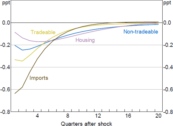
Figure 11 shows the response of sectoral inflation to the monetary policy shock. Housing services inflation has the smallest but the most persistent response. While this seems somewhat at odds with the fact that housing investment and output are reasonably sensitive to changes in the cash rate, the muted response of housing services inflation reflects two offsetting factors. On the one hand, lower aggregate demand places downward pressure on the price of housing services. On the other hand, the large fall in housing investment, and associated decrease in the housing stock, places upward pressure on prices. Thus, the overall response of housing services inflation is muted. Conversely, the price of imported goods and services declines substantially on impact. This is mainly due to the exchange rate appreciation induced by higher interest rates. Inflation decreases mildly in the tradeable and non-tradeable sectors.
Note: 100 basis point increase in cash rate
Note: 100 basis point increase in cash rate
4.2 Empirical Evidence from SVARs
As shown above, our model and RSH have slightly different dynamic predictions. This raises two related questions:
- To what extent are these differences a natural consequence of analysing more disaggregated data?
- To the extent that they reflect modelling choices, do our modelling choices help us to match the observed data?
We attempt to answer these questions by studying the dynamics implied by the more disaggregated data in a much less structured environment – SVARs. In particular, we estimate a series of SVARs using a subset of the same data we use in estimating the DSGE model and compare the impulse responses implied by the SVARs to those implied by the DSGE model.
4.2.2 The SVAR model
We assume that the economy can be represented using the following structural form:
where the matrix B summarises the contemporaneous relationships between the variables; C(L) is an autoregressive lag polynomial of order L, which summarises how the variables are affected by their own lags as well as the lags of the other variables in the system; and ut is a vector of independently and identically distributed structural shocks. The vector Xt contains foreign and domestic variables. We assume that the foreign variables are block exogenous: domestic variables cannot affect the foreign variables either contemporaneously or with a lag. This is consistent with other SVAR models of the Australian economy, where Australia is modelled as a small open economy (e.g. Manalo, Perera and Rees 2014). The foreign variables are the same ones we include in the DSGE model: commodity prices ( ); a measure of global economic activity (
 ); the average foreign inflation rate (
 ); and the average foreign policy rate (
 ). The domestic variables mimic a cut down version of the domestic economy from the DSGE model, and include: a set of GDP components (discussed below) denoted by
  ; trimmed mean inflation (πt); the cash rate (rt); and the real trade-weighted exchange rate (qt). Thus, the full vector
  .
.
As in the DSGE model, all variables are quarterly growth rates except the foreign and domestic policy rates, which are expressed in percentage points, and the sample runs from 1992:Q1 to 2016:Q4. We include three separate dummy variables in the model to account for: the introduction of inflation targeting (1992:Q1–1992:Q4); the introduction of the goods and services tax (2000:Q2–2000:Q3) and the global financial crisis (2008:Q4–2009:Q3). Considering the large number of variables included in the model, and for consistency across the results, we estimate all specifications with two lags (Liu, Pagan and Robinson (2018) show that such a lag length is sufficient to capture the dynamics of the RSH model).
We identify monetary policy shocks using a recursive ordering approach, where each variable in Xt can contemporaneously affect only variables later in the ordering.[20] Our ordering implies that shocks to real activity and inflation contemporaneously affect the cash rate. However, changes in the cash rate affect the other macroeconomic variables with a lag. This is a standard identification assumption of monetary policy shocks and reflects that fact that it takes time for economic agents to alter pricing, production and spending decisions in response to changed monetary policy conditions.[21]
4.2.3 SVAR results
We estimate four separate SVARs, which differ from each other in the way in which we decompose aggregate output growth. Specifically, we decompose aggregate output growth either into its expenditure components or into gross value-added production in the different sectors of the economy. For both decompositions, we estimate one SVAR where we separate out housing, and one where we do not. The GDP components included in each specification are summarised in Table 6.
| Model | Components |
|---|---|
| Model 1 | Tradeable sector value added, non-tradeable sector value added, resource sector value added |
| Model 2 | Tradeable sector value added, non-tradeable sector (excluding housing) value added, housing sector value added, resource sector value added |
| Model 3 | Consumption, investment, exports, imports |
| Model 4 | Consumption, investment (excluding housing), housing investment, exports, imports |
The models that separate out housing are similar in structure to our DSGE model, while the models that do not split out housing are similar in structure to the model in RSH. Therefore, by comparing the responses of the variables to a monetary policy shock across the SVAR models, we can gauge the importance of explicitly accounting for the housing sector. Moreover, we can also assess whether our assumption that housing investment is more interest sensitive is borne out in the data.
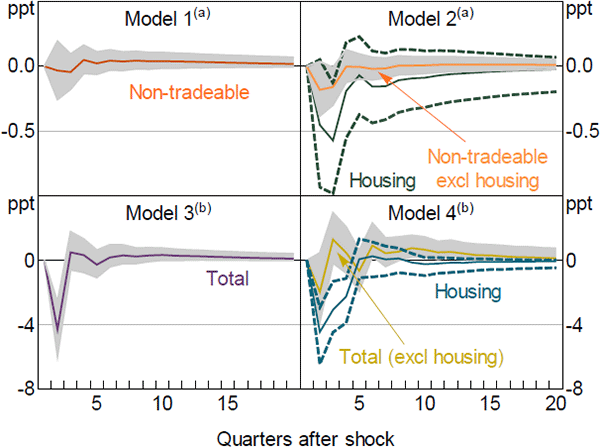
Figure 12 shows the responses of selected variables to an exogenous 100 basis point increase in the cash rate, along with the 68 per cent confidence bands. In Model 1, the response of value-added growth in the non-tradeable sector is very small and is not statistically significant. However, if we split the housing sector out, as we do in Model 2, the negative response of growth in value added for the non-tradeable (excluding housing) sector is larger and more persistent, although still not statistically significant. Value-added growth in the housing sector declines by almost 0.6 percentage points. Although the confidence intervals around this response are wide, the decrease in housing value-added growth is statistically significant after two quarters.
Notes:
100 basis point increase in cash rate
(a) Sector value added
(b) Investment
While it might seem surprising that the responses are larger for both sectors in Model 2, the finding is broadly consistent with Lawson and Rees (2008). They estimate an SVAR of the Australian economy including the expenditure components of GDP, and find that the implied aggregate response of GDP from this model is larger and more persistent than the response from a model estimated using aggregate GDP (in place of the expenditure components). Both sets of findings suggest that aggregating across sectors leads to a loss of useful information, which reinforces the importance of separately modelling the housing sector in the DSGE model.
Looking at the models that include the expenditure components of GDP, using Model 3 we find a statistically significant decline in total investment growth of about 4 percentage points in response to the monetary policy shock. However, if we decompose total investment into the housing and total excluding housing components, as we do in Model 4, it is evident that the aggregate response is largely driven by dwelling investment. This is consistent with the dynamic predictions of our model, and supports our decision to calibrate investment adjustment costs in the non-housing sectors to be relatively high.
It is worth noting that while the SVAR results are qualitatively similar to those from the DSGE model, quantitatively there are some substantial differences. In particular, the responses of housing investment and value added are much larger in the SVAR. However, given the large confidence bands around the SVAR's estimated responses, as well as the simple identification scheme used, we prefer to focus on the qualitative results.
5. The Transmission of Housing Shocks
As shown above, adding a housing sector to the existing DSGE model helps us to match certain patterns in the data, such as the relative responsiveness of housing investment to monetary policy shocks. Another benefit is that it also allows us to examine how shocks to the housing sector are transmitted through the economy.
The housing sector features a number of shocks that, for the sake of interpretation, we split into two classes: shocks to the stock of housing, such as housing preference shocks and housing investment shocks; and shocks to housing services, such as shocks to productivity in the housing services sector. We study below the model-implied responses of the endogenous variables to each of these shocks and compare where appropriate to the predictions of the canonical model of Iacoviello and Neri (2010).
5.1 Shocks to the Housing Stock
In the model, negative housing investment shocks imply that agents need to use up more consumption goods to produce a given quantity of new housing stock. In this sense, it is very similar to the housing technology shocks in Iacoviello and Neri (2010). While the shock directly implies some exogenous increase in construction costs, it can more generally be interpreted as some exogenous shock that lowers the level of housing investment.
Figure 13 shows the response of selected variables to a housing investment shock that lowers housing investment by 5 per cent. The lower housing investment, and so lower demand for intermediate goods, causes GDP to fall by about ½ per cent. Total investment and consumption also fall. The latter is in contrast to Iacoviello and Neri (2010), who find that consumption rises in response to a negative housing (investment) technology shock. The difference reflects the fact that in Iacoviello and Neri, housing and other consumption are substitutes (abstracting from collateral effects), in that agents can raise their utility by consuming more of one or the other. While this is also the case in our model, the fact that the housing capital stock is used to produce housing services, which make up part of the consumption bundle, creates an offsetting ‘complimentary’ relationship between the housing stock and consumption.
On the nominal side, inflation declines slightly and the cash rate is lowered by around 10 basis points. The modest fall in inflation is the result of offsetting forces in the economy. The contraction in housing investment supports the housing-related components of inflation by lowering the supply of housing, while the decreased demand for intermediate goods lowers inflation in the non-tradeable and tradeable sectors (Figure 14). The combined effect is a modest fall in overall inflation.
Housing preference shocks are exogenous shocks to the demand for the stock of housing which allow for a greater gap between the rate of return on housing and that on other capital. Such shocks can be interpreted in different ways, including as: a change in the taxation treatment of housing; a change in expectations regarding future capital gains on housing; or a change in demand from foreign buyers.[22]
Figure 13 also shows the response of selected variables to a housing preference shock that causes a 5 per cent decline in housing investment. The responses are very similar to those for a housing investment shock. This does suggest that the model may have difficulties separately identifying these two shocks, which is somewhat reflected in our estimation results where we observe some signs of weak identification for the preference shock parameters. Nevertheless, we include both in the model as they are likely to have quite different implications if we consider anticipated shocks in scenario analysis.
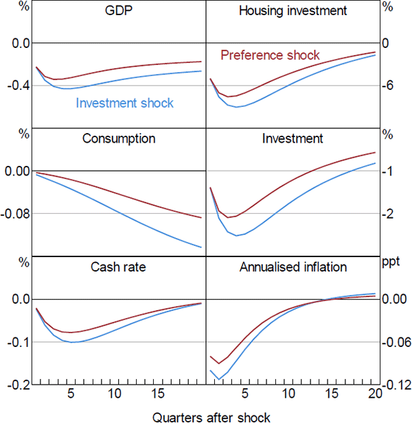
Note: 5 per cent decline in housing investment
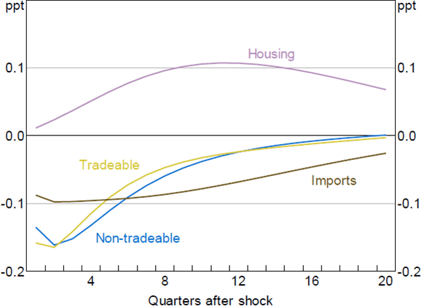
Note: 5 per cent decline in housing investment
In both cases, households will have an incentive to decrease investment in advance of the negative shock due to the investment adjustment costs and, to a lesser extent, habit persistence in the housing capital stock in households' utility functions. But, in the case of an investment shock, they will have an offsetting incentive to increase investment immediately, when it is relatively ‘cheap’. As such, the magnitude and dynamics of the investment response will differ somewhat in the two cases.[23] Therefore, having both shocks enables us to perform a more diverse range of scenario analyses.
The responses to the housing preference shock in our model are also qualitatively similar to those for a housing preference shock in Iacoviello and Neri (2010). In their baseline model, consumption declines following a negative housing preference shock. However, in their model without collateral constraints, consumption rises. Our model, which also does not include collateral constraints, matches their baseline model, which includes collateral constraints. Therefore, our specification can match some of the qualitative predictions arising from a more complex model with heterogeneous agents and a banking system.
5.2 Shocks to Housing Services
Our model also allows for exogenous changes in the productivity of the housing services sector. That is, more or less housing services being produced with the same level of housing stock and labour. This could, for example, capture changes in the composition of the housing stock such as a shift towards apartments or smaller houses, that produce more housing services per dollar of housing stock. There is no equivalent shock in the Iacoviello-type framework.
Figure 15 shows the responses of selected variables to a technology shock that lowers housing investment by 5 per cent. Lower productivity in the housing services sector leads to lower production and investment in that sector, and in aggregate. It also pushes up prices of housing services substantially, which flow through to higher aggregate inflation and therefore a higher cash rate.
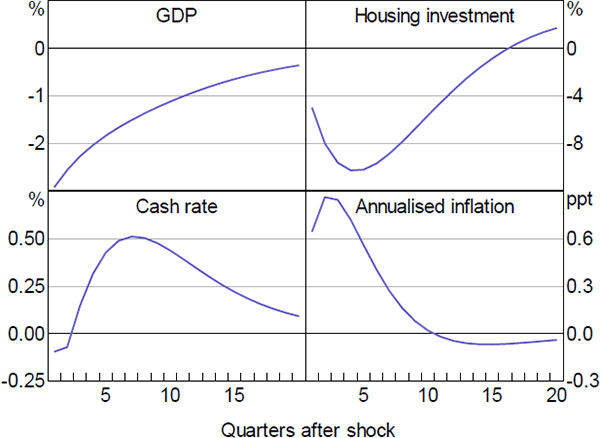
Note: 5 per cent decline in housing investment
6. Housing and Australia's Post Mining Boom Transition
In this section, we use the model to assess the role of housing investment in supporting economic activity since the end of the mining boom in 2012. The DSGE model provides us with two ways to assess how important activity in the housing sector was in helping the rebalancing of the economy. The first is to use a historical decomposition to quantify how much of the recent increase in housing investment is related to lower commodity prices, and in particular to lower interest rates associated with these lower prices. The second is to run a counterfactual scenario where housing sector activity does not pick up after the end of the mining boom.
6.1 Historical Decomposition
The idea behind a historical decomposition is as follows. The model attributes all deviations of the observable variables from their steady-state values to the model's structural shocks. A historical decomposition recovers these shocks and therefore allows us to single out which structural shocks have been driving a given variable of interest.
The model interprets fluctuations in commodity prices over the cycle as a series of positive and negative commodity price shocks. In order to examine the response of housing investment to the end of the mining boom we therefore focus on commodity price shocks.
In the model, a key channel through which commodity price shocks affect housing investment is by influencing interest rates. As commodity prices fall, disinflationary pressures lead the central bank to lower interest rates, which in turn stimulates housing investment.[24] We refer to this effect as the ‘endogenous’ interest rate channel. This channel reflects how the central bank responds to broader macroeconomic consequences of the fall in commodity prices, that is, falls in inflation, output, and employment. To the extent that the central bank takes other factors into consideration, this will show up in the model as monetary policy shocks.
Commodity price shocks consistently weighed on housing investment during the 2000s and continued to do so until the peak of the terms of trade in 2012 (Figure 16). This reflects the endogenous response of interest rates to the expansionary impulse, and more generally the flow of inputs towards mining activities and investment. More recently, as commodity prices have fallen, the opposite forces have been at work. This is consistent with the notion that housing investment has stepped in to fill the void left by the mining boom and to assist in the economic transition.
Meanwhile, monetary policy shocks have consistently made positive contributions to housing investment since 2013. This indicates that monetary policy has been looser than the model predicts based on its estimated relationships and the observables. In this sense, monetary policy has provided additional help in the transition of the economy. We note, however, that in recent years the independent contribution of monetary policy shocks has declined relative to that of commodity price shocks. One potential explanation for these dynamics is that monetary policy is more forward looking than is implied by the model specification. To the extent that policymakers expected future declines in commodity prices to weigh on future inflation and growth, they may have responded pre-emptively. The model would interpret this pre-emptive action as monetary policy shocks, even if it was related to (future) commodity price shocks.
Taken together, the above results suggest that the housing investment boom we have observed in recent years was largely a ‘natural’ response of the Australian economy to the large fall in commodity prices. Even in the absence of all monetary policy shocks, the model still predicts large increases in housing investment as a response to the end of the mining boom.
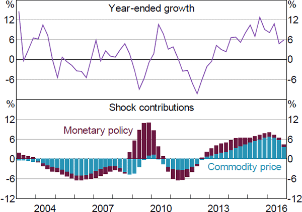
Sources: ABS; Authors' calculations
In this context, it is also worth considering the role of other shocks in the evolution of housing investment. Aside from commodity price and monetary policy shocks, the model also suggests that housing investment shocks have played an important role in determining housing investment in recent years. However, somewhat surprisingly the model suggests that housing investment shocks have weighed on housing investment. That is, housing investment has been somewhat weaker than the model would predict given the prevailing macroeconomic conditions. One potential explanation could be capacity constraints in the housing construction industry, which the (linear) model is not able to adequately capture. It is also possible that changes in lending standards could have weighed on investment.
6.2 Counterfactual Scenario
As noted above, another way to assess the importance of the housing sector in aiding Australia's economic transition is to use a counterfactual scenario. Specifically, we run a scenario where housing investment and value added continued growing at their mining boom averages, rather than accelerating. For the counterfactual, we define the mining boom as March quarter 2003 to June quarter 2012.
We start by taking the structural shocks estimated using a historical decomposition, discussed above. With these shocks in hand, we can then look at our counterfactual while incorporating all of the shocks that would have hit the economy over the period.
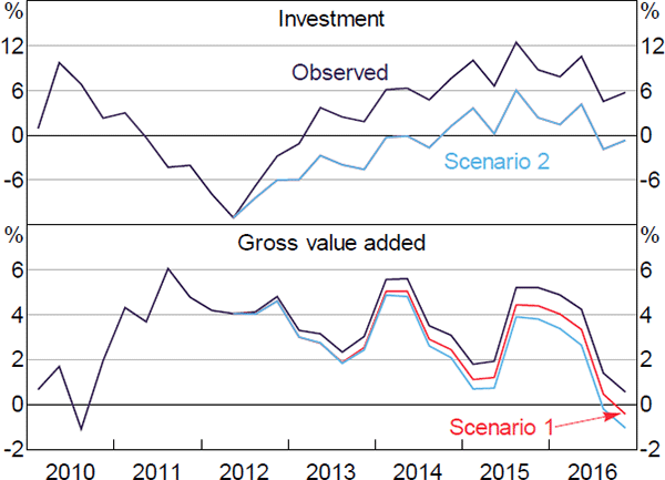
Table 7 shows the averages of quarterly growth in housing investment and housing sector value added over the boom and post-boom periods. We use these averages to produce two different scenarios. In the first, we lower quarterly housing investment growth by 1.6 percentage points for each quarter in the post-boom period. We do so using shocks to housing investment. In the second, we also incorporate housing sector-specific technology shocks so that quarterly growth in housing sector value added is, on average, 0.2 percentage points below its actual history.[25],[26] The resulting calibrations for these scenarios are shown in Figure 17 (note housing investment is the same in scenarios 1 and 2).
| Housing investment | Housing sector value added | |
|---|---|---|
| Boom: 2003:Q1–2012:Q2, per cent | 0.0 | 0.6 |
| Post-boom: 2012:Q3–2016:Q4, per cent | 1.6 | 0.8 |
| Difference, percentage points | 1.6 | 0.2 |
Sources: ABS; Authors' calculations
Figure 18 compares the observed growth in GDP and inflation to our scenarios. Under the scenarios, year-ended GDP growth is around ½ percentage point lower. Inflation is also somewhat lower; however, disinflationary pressures from softer growth are partly offset by higher inflation in the housing sector due to the smaller and less productive housing stock. Under both scenarios, the cash rate is around 40 basis points lower.
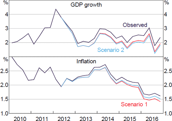
Sources: ABS; Authors' calculations
These estimates potentially understate the importance of the housing sector in the economy's transition. The model does not include borrowing, and therefore cannot account for any loosening of collateral constraints associated with the strong housing price growth witnessed in some cities over recent years. Similarly, as we model the price of housing services, not of the housing stock, the model may not adequately account for wealth effects associated with said housing price growth. Moreover, the model assumes that all investment is done using the final consumption good. This does not allow the inputs into different types of investment to differ. To the extent that the inputs used in mining investment are more similar to those used in residential construction than to those used in (for example) machinery and equipment investment, the housing sector may play a more important role in smoothing the economy's transition away from mining than the model indicates.
7. Conclusion
Motivated by the recent increase in housing investment, we extend the DSGE model constructed by RSH to include a standalone housing sector. In doing so, we outline a simple way to incorporate a housing sector into a multi-sector DSGE model that has several appealing features, including its focus on modelling housing services (which have a large weight in GDP and the CPI basket). Moreover, we show that it can qualitatively match a number of the predictions of more complicated models with heterogeneous agents and borrowing.
Our new model provides predictions that are broadly consistent with those from RSH. However, using impulse response analysis we have shown how the propagation of key macroeconomic shocks has changed in the housing-augmented model. In particular, housing investment is more responsive to monetary policy shocks than is other investment. As discussed, this is due in part to calibration choices and in part to our utility specification, and is consistent with SVAR evidence.
We also show how the new model can be used for the exploration of housing-related scenarios, such as examining the drivers of housing investment since the end of the mining boom. The ability to use the model for such analyses means that it constitutes a useful addition to the Bank's suite of models.
Appendix A: Data Sources for Estimation
GDP: Quarterly percentage change of real gross domestic product, seasonally adjusted and in chain volume terms. Source: ABS Cat No 5206.0 ‘Australian National Accounts: National Income, Expenditure and Product’.
Consumption: Quarterly percentage change of real household final consumption expenditure, seasonally adjusted and in chain volume terms. Source: ABS Cat No 5206.0.
Investment: Quarterly percentage change of real private gross fixed capital formation, seasonally adjusted and in chain volume terms. Source: ABS Cat No 5206.0.
Housing investment: Quarterly percentage change of real private dwelling investment (gross fixed capital formation), seasonally adjusted and in chain volume terms. Source: ABS Cat No 5206.0.
Public demand: Quarterly percentage change of real public demand. Public demand is calculated as the sum of government final consumption expenditure and public gross fixed capital formation, with all data seasonally adjusted and in chain volume terms. Source: ABS Cat No 5206.0.
Hours worked: Quarterly percentage change in hours worked, seasonally adjusted. Source: ABS Cat No 5206.0.
Resource exports: Quarterly percentage change in resource export volumes, seasonally adjusted and in chain volume terms. Source: RBA statistical table I1 International Trade and Balance of Payments.
Non-resource exports: Quarterly percentage change in non-resource export volumes. Non-resource export volumes are calculated as the difference between total export volumes and resource export volumes, with all data in seasonally adjusted and in chain volume terms. Source: RBA statistical table I1.
Non-tradeable excluding housing value added: Quarterly growth rate of value-added production in the non-tradeable sector. The non-tradeable sector consists of the following industries: electricity, gas, water & waste; retail trade; information, media & telecommunications; finance & insurance; professional services; administrative services; public administration; education industry; healthcare; arts & recreation; and other services. Part of the construction industry is apportioned to this sector, based on the share of total construction work done that is non-residential. We calculate the growth rate of this series by summing the growth rates of each industry weighted by that industry's share of non-tradeable excluding housing value added. Sources: ABS Cat No 5204.0 ‘Australian System of National Accounts’, ABS Cat No 8755.0 ‘Construction Work Done, Australia, Preliminary’ and ABS Cat No 5206.0.
Housing value added: Quarterly growth rate of value-added production in the housing sector. The housing sector consists of the real estate industry and ownership of dwellings. Part of the construction industry is apportioned to this sector, based on the share of total construction work done that is residential. We calculate the growth rate of this series by summing the growth rates of each industry weighted by that industry's share of housing. Sources: ABS Cat Nos 5204.0, 8755.0 and 5206.0.
Non-resource tradeable value added: Quarterly growth rate of value-added production in the non-resource tradeable sector. The non-resource tradeable sector consists of the following industries: agriculture, forestry & fishing; manufacturing; transport; wholesale trade; and accommodation & food services. We calculate the growth rate of this series by summing the growth rates of each industry weighted by that industry's share of non-resource tradeable value added. Sources: ABS Cat Nos 5204.0 and 5206.0.
Resource value added: Quarterly growth rate of value-added production in the mining industry. Source: ABS Cat No 5206.0.
Inflation: Quarterly trimmed mean inflation excluding interest and tax changes. Source: RBA statistical table G1 Consumer Price Inflation.
Housing sector inflation: Quarterly inflation in housing-related components of the CPI, including: rents, home maintenance & repairs; home insurance; and new purchases by owner occupiers. Weighted using ABS's Consumer Price Index Weighting Patterns (various releases). Seasonally adjusted using seasonal factors released by the ABS. Source: ABS Cat No 6401.0 ‘Consumer Price Index, Australia’.
Non-tradeable excluding housing inflation: Quarterly inflation in non-housing-related non-tradeable components of the CPI. For details on inclusions see RBA (2014). Weighted using ABS's Consumer Price Index Weighting Patterns (various releases). Seasonally adjusted using seasonal factors released by the ABS. Source: ABS Cat No 6401.0.
Tradeable inflation: Quarterly growth in the services credits implicit price deflator, seasonally adjusted. ABS Cat No 5302.0.
Sectoral wages: Quarterly growth in the wage price index for each sector. Industry allocation to sectors is the same as for value added. We calculate the growth rate of the series by summing the growth rates of each industry weighted by that industry's share of total sectoral hours. All data are seasonally adjusted. Sources: ABS Cat No 6345.0 ‘Wage Price Index, Australia’ and ABS Cat No 6291.0.55.003 ‘Labour Force, Australia, Detailed, Quarterly’.
Cash rate: Quarterly average cash rate target. Source: RBA statistical table F1.1 Interest Rates and Yields – Money Market.
Nominal exchange rate: Quarterly average percentage change in the nominal trade-weighted exchange rate. Source: RBA statistical table F11 Exchange Rates.
Resource prices: Quarterly average percentage change in the RBA non-rural commodity price index measured in Special Drawing Rights. Source: RBA statistical table I2 Commodity Prices.
Foreign GDP: Quarterly percentage change of the real gross domestic product of Australia's major trading partners weighted by export share. Source: RBA.
Foreign inflation: Quarterly average inflation rate of Australia's major trading partners weighted by export share. Source: RBA.
Foreign interest rates: Quarterly average policy rate of the United States, Japan and euro area (Germany before 1999). Source: RBA statistical table F13 International Official Interest Rates.
Appendix B: Transmission of Commodity Price Shocks
We analyse the effects of a 10 per cent increase in commodity prices on real GDP and inflation, which are shown in Figure B1. Higher commodity prices lead to an expansion in the economy; real GDP increases to be around 0.35 per cent above its baseline level. The increase is similar to that predicted by the RSH model. The response of inflation, though, is larger in our model, at least initially, but quickly decays to near zero. Both models' inflation responses are somewhat consistent with Jääskelä and Smith (2013) and Downes, Hanslow and Tulip (2014), who show that higher commodity prices lead to small or even negative responses of inflation.
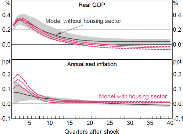
Note: 10 per cent increase in commodity prices
The responses of sectoral investment and value added are shown in Figure B2. Higher commodity prices lead to increased production in the resource sector. Value added in the housing sector increases, which partly reflects increases in domestic income, while non-tradeable value added is mostly unchanged. Meanwhile, value added in the tradeable sector contracts as the increase in resource prices causes an appreciation of the real exchange rate, making the sector less competitive.
As expected, the expansion in investment is concentrated in the resource sector. The increase, however, occurs slowly: the peak response occurs three years after the shock with resource investment around 3 per cent above baseline. This is consistent with the observation that mining investment was relatively slow to respond to the increase in commodity prices in the mid 2000s (peaking after the peak in the terms of trade). In the housing sector, investment falls moderately. This contraction reflects a mild increase in the cash rate in response to the temporary expansion in activity, as well as increased relative returns to investment in mining capital.
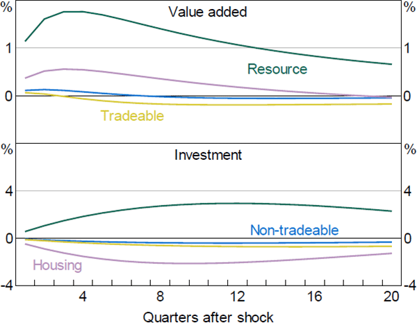
Note: 10 per cent increase in commodity prices
Looking at sectoral inflation (Figure B3), the appreciation in the nominal exchange rate causes a large fall in the rate of inflation of imported goods and services. At the same time, increased domestic demand pushes up prices in other sectors. In aggregate, these responses offset each other to a degree and the overall inflation rate remains muted after the shock, as shown in Figure B1. This is largely consistent with the sectoral response found in the RSH model.
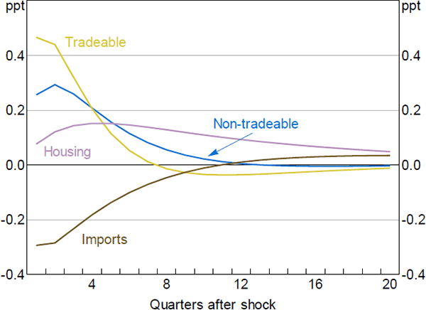
Note: 10 per cent increase in commodity prices
Appendix C: Transmission of Exchange Rate Shocks
The aggregate effect of an unanticipated 10 per cent appreciation of the nominal exchange rate is shown in Figure C1. Our model predicts a slightly larger and more persistent decline in GDP compared to RSH. The fall in economic activity in both models is driven by a decrease in net exports as the appreciation makes exports less competitive abroad and imports more competitive domestically. Consistent with this, the falls in value added are larger in the more trade-exposed sectors: resource and tradeable (Figure C2). The exchange rate appreciation causes a decline in inflation that is slightly larger in magnitude compared to that in the RSH model. The decline largely reflects lower prices for imported goods.
In response to the fall in inflation and output, the central bank lowers the cash rate, which causes an increase in investment (Figure C2). The response of housing investment is quite large, peaking at around while 3 per cent, while the remaining sectors' investment are broadly unchanged. The difference reflects the greater sensitivity of housing investment to changes in the interest rate.
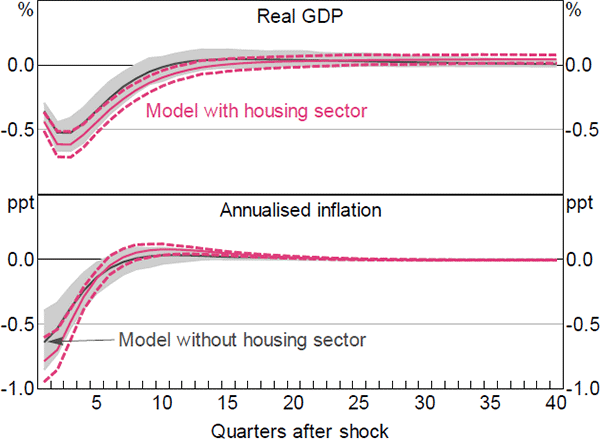
Note: 10 per cent appreciation of nominal exchange rate
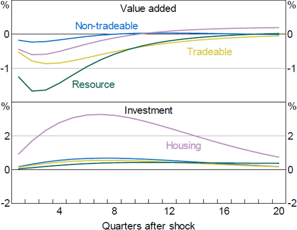
Note: 10 per cent appreciation of nominal exchange rate
References
An S and F Schorfheide (2007), ‘Bayesian Analysis of DSGE Models’, Econometric Reviews, 26(2–4), pp 113–172.
Berkelmans L (2005), ‘Credit and Monetary Policy: An Australian SVAR’, RBA Research Discussion Paper No 2005-06.
Brooks SP and A Gelman (1998), ‘General Methods for Monitoring Convergence of Iterative Simulations’, Journal of Computational and Graphical Statistics, 7(4), pp 434–455.
Burgess S, E Fernandez-Corugedo, C Groth, R Harrison, F Monti, K Theodoridis and M Waldron (2013), ‘The Bank of England's Forecasting Platform: COMPASS, MAPS, EASE and the Suite of Models’, Bank of England Working Paper No 471.
Downes P, K Hanslow and P Tulip (2014), ‘The Effect of the Mining Boom on the Australian Economy’, RBA Research Discussion Paper No 2014-08.
Dvornak N and M Kohler (2007), ‘Housing Wealth, Stock Market Wealth and Consumption: A Panel Analysis for Australia’, Economic Record, 83(261), pp 117–130.
Fox R and R Finlay (2012), ‘Dwelling Prices and Household Income’, RBA Bulletin, December, pp 13–22.
Gillitzer C and JC Wang (2015), ‘Housing Wealth Effects: Cross-Sectional Evidence from New Vehicle Registrations’, RBA Research Discussion Paper No 2015-08.
Iacoviello M (2005), ‘House Prices, Borrowing Constraints, and Monetary Policy in the Business Cycle’, The American Economic Review, 95(3), pp 739–764.
Iacoviello M and S Neri (2010), ‘Housing Market Spillovers: Evidence from an Estimated DSGE Model’, American Economic Journal: Macroeconomics, 2(2) pp 125–164.
Jääskelä JP and P Smith (2013), ‘Terms of Trade Shocks: What Are They and What Do They Do?’, Economic Record, 89(285), pp 145–159.
Komunjer I and S Ng (2011), ‘Dynamic Identification of Dynamic Stochastic General Equilibrium Models’, Econometrica, 79(6), pp 1995–2032.
Kulish M and D Rees (2011), ‘The Yield Curve in a Small Open Economy’, Journal of International Economics, 85(2), pp 268–279.
Lawson J and D Rees (2008), ‘A Sectoral Model of the Australian Economy’, RBA Research Discussion Paper No 2008-01.
Lim G and S Tsiaplias (2016), ‘Non-Linearities in the Relationship between House Prices and Interest Rates: Implications for Monetary Policy’, Melbourne Institute Working Paper No 2/16.
Liu X, AR Pagan and T Robinson (2018), ‘Critically Assessing Estimated DSGE Models: A Case Study of a Multi-Sector Model’, Australian National University Crawford School of Public Policy, Centre for Applied Macroeconomic Analysis, CAMA Working Paper 4/2018.
Lowe P (2015), ‘Managing Two Transitions’, Address given at the Corporate Finance Forum, Sydney, 18 May.
Manalo J, D Perera and D Rees (2014), ‘Exchange Rate Movements and the Australian Economy’, RBA Research Discussion Paper No 2014-11.
Muellbauer J (2015), ‘Housing and the Macroeconomy: Inflation and the Financial Accelerator’, Journal of Money, Credit and Banking, 47(S1), pp 51–58.
Nakajima M and IA Telyukova (2013), ‘Housing in Retirement across Countries’, Center for Retirement Research at Boston College Working Paper No 2013-18.
Ramey VA (2016), ‘Macroeconomic Shocks and Their Propagation’, in JB Taylor and H Ulhig (eds), Handbook of Macroeconomics: Volume 2A, Handbooks in Economics, North-Holland, Amsterdam, pp 71–162.
Rayner V and J Bishop (2013), ‘Industry Dimensions of the Resource Boom: An Input-Output Analysis’, RBA Research Discussion Paper No 2013-02.
RBA (Reserve Bank of Australia) (2014), ‘Box B: Inflation and the Housing Cycle’, Statement of Monetary Policy, November, pp 55–57.
RBA (2015), ‘Box C: The Cycle in Dwelling Investment’, Statement on Monetary Policy, May, pp 43–45.
Rees D, P Smith and J Hall (2016), ‘A Multi-Sector Model of the Australian Economy’, Economic Record, 92(298), pp 374–408.
Rotemberg JJ (1982), ‘Sticky Prices in the United States’, Journal of Political Economy, 90(6), pp 1187–1211.
Shoory M (2016), ‘The Growth of Apartment Construction in Australia’, RBA Bulletin, June, pp 19–26.
Skinner JS (1996), ‘Is Housing Wealth a Sideshow?’, in DA Wise (ed), Advances in the Economics of Aging, NBER Project Report, University of Chicago Press, Chicago, pp 241–268.
Smets F and R Wouters (2007), ‘Shocks and Frictions in US Business Cycles: A Bayesian DSGE Approach’, The American Economic Review, 97(3), pp 586–606.
Sutton M (2017), ‘The Average Size and Proportion of Price Changes in the CPI’, in ‘Consumer Price Index, Australia, September Quarter 2017’, ABS Cat No 6401.0, pp 12–21.
Acknowledgements
The authors would like to thank Daniel Rees, Tim Robinson, Gian-piero Lovicu, Jarkko Jääskelä, John Simon, participants of the Sydney Macro Reading Group Workshop and seminar participants at the Australian Treasury and the Australian National University for helpful comments. The views expressed in this paper are those of the authors and do not necessarily reflect the views of the Reserve Bank of Australia. The authors are solely responsible for any errors.
Footnotes
UNSW Sydney [*]
Economic Research Department, Reserve Bank of Australia [**]
See, for example, Fox and Finlay (2012), RBA (2015), Lim and Tsiaplias (2016) and Shoory (2016), among others. [1]
Iacoviello (2005) and Iacoviello and Neri (2010) both use aggregate consumption data as an observable for consumption excluding housing, which creates an inconsistency between model variables and their real world counterparts. Moreover, both papers focus on the quantity and price of the housing stock, not housing services, with the latter being the relevant concept for GDP and CPI inflation. [2]
The current weight of the housing component of the CPI basket is about 23 per cent. The average housing share of nominal gross value added from 1993 to 2016 is around 16 per cent. [3]
Interest on ‘margin loans’ used to purchase equities is treated similarly to interest on housing loans. However margin lending is much less prevalent. [4]
Similar complicated tax arrangements exist across the developed world and typically are not modelled in DSGE settings. [5]
It is worth noting that our model can be further extended to incorporate heterogeneous households and borrowing constraints. This is an important task for future research. [6]
We follow RSH and assume that the risk premium shock, ψt, depends on the stock of foreign debt outstanding such that  , where νt follows an autoregressive process.
[7]
We assume that F is a function of the steady-state growth rate of labour-augmenting productivity, μ, such that  and
and  . In practice, we adopt the following function form:
  .
[8]
.
[8]
For a detailed description of each individual sector we direct the interested reader to RSH. [9]
Despite land being included in the model as part of the mining production function, we do not include land as a factor of production for the housing sector. Instead, to retain a close link to the original model and to the production of other non-tradeable goods, we choose the same functional form for the production function as that of the non-tradeable sector. Considering a fixed factor here is an interesting area to explore in future iterations of the model. [10]
The calibration parameters for this exercise are β = 0.95, μ = 1.008, bd = 0.15, Ad = 0.3, and λd = 1. [11]
In steady state, the real interest rate is pinned down by the household discount factor, β. That is, for a given value of the discount factor the steady-state real interest rate is such that households are indifferent between consumption today and consumption in the future. Increases in β correspond to decreases in the steady-state value of the real rate of interest since the value of future consumption rises relative to that of current consumption. [12]
Unless otherwise noted, we use the same calibrated parameters in the foreign economy as in the domestic economy. For example, the discount rate β is set to the same value in both economies. [13]
As we include errors in the inflation and GDP components, we do not also include them in the aggregates. [14]
We have tried a number of different measurement error specifications, including moving average unit root processes for key aggregate and foreign variables, white noise errors included on all observables, and the removal of all such error terms from the model. We find that, at a minimum, some error terms must be included in the sector-specific level variables in order for the model to be estimated. This is due to the non-additivity of chain volume measures and definitional incongruences between sectoral observables and their model counterparts. However, we find that the precise specification of these terms does not have a significant impact on the inference of estimated parameters once some error is included at the sectoral level. Therefore, we chose the most parsimonious specification. [15]
We set the world economy parameters to the mean values of the posterior distribution. [16]
Graphical evidence suggests the number of draws is sufficient to ensure convergence. We obtain an acceptance rate of about 30 per cent. [17]
Since the model calibrations and assumed priors are based on the full sample, the DSGE model is not at a complete informational disadvantage. [18]
In Appendices B and C we compare the responses between the two models for commodity price and exchange rate shocks, respectively. [19]
For an overview of different methods for identifying monetary policy shocks, see Ramey (2016). [20]
As pointed out by our referees, our DSGE model is unlikely to be recursive. This means that there isn't a direct mapping from our DGSE model to the SVAR model specified in this section. We note, however, that our intent is not to estimate the VAR representation of our DSGE model. Rather, our aim is to show that the DSGE model results are consistent with evidence arising from a much less structured model. We do not explore alternative VAR identification strategies, such as sign restrictions, as our exercise here is intended to be illustrative. [21]
In interpreting the shock as a change in demand from foreign buyers, we would be abstracting from any potential exchange rate effects stemming from changes in capital inflows and outflows. [22]
The degree of difference will depend on a number of factors, including: the degree of habit persistence; the size of the investment adjustment costs; how far in the future the anticipated shock will occur; and the size and duration of the shock. [23]
Jääskelä and Smith (2013) find that increases in the terms of trade are not always associated with inflationary pressures and higher interest rates. Our commodity price shock is most similar to their world demand shock, which is associated with higher domestic interest rates. [24]
As these housing technology shocks weigh on housing investment, the housing investment shocks required to hit our target for housing investment are smaller than in scenario 1. [25]
We choose technology shocks as apartments have made up a particularly large portion of recent residential construction (e.g. Shoory 2016). In some sense, this can be seen as a positive technology shock, as a given amount of investment produces more dwellings and housing services compared to construction of single-family dwellings. This type of interpretation is supported by the historical decomposition, which shows that improved productivity in the housing services sector has supported value-added growth. [26]


