RDP 2015-02: Central Counterparty Loss Allocation and Transmission of Financial Stress 3. Data and Exposure Analysis
March 2015 – ISSN 1448-5109 (Online)
- Download the Paper 1.26MB
The first step in exploring the question of how collateralisation and CCP clearing affect the stability of a financial system is to construct a matrix of bilateral positions between counterparties.
To do this, we use data on the total derivative assets and liabilities of 41 financial institutions across 5 categories of OTC derivatives at the end of 2012. These data were compiled for the Macroeconomic Assessment Group on Derivatives (MAGD 2013). The original data, and the transformations that we use to create a matrix of bilateral net notional positions, are described in Section 3.1.
The next step is to derive the bilateral exposure matrices, which are a function of the bilateral positions and the opportunities for netting. As noted, the scope for netting will depend on the extent to which transactions are cleared non-centrally, through a single CCP, or through separate CCPs for each asset class. The set of clearing arrangements that we consider is described in Section 3.2. To illustrate the dataset and establish some stylised facts that are relevant for the analysis in the remainder of the paper, we also present and discuss how exposures and collateral requirements change under each alternative clearing arrangement.
3.1 The Dataset and the Position Matrix
The data used in this analysis were compiled by the MAGD and consist of reported balance sheet data for 41 banks that are involved in OTC derivative trading. Of the 41 banks, 16 are widely recognised as forming the ‘core’ of the OTC derivative markets. The remaining 25 banks were chosen because they participate in OTC derivative markets, interact with CCPs, and/or are large regional banks (MAGD 2013, Table 3). These banks are typically smaller and are more likely to be involved in OTC derivative markets as part of their client business rather than as dealers with a market-making role. We have not included non-banks or any non-financial institutions (end users) in this network.
For B banks, we define the OTC derivative obligations owed by bank i
to bank j in product-class k to be  . Bank i's
total derivative liabilities in product-class k will be given by the
sum of its obligations to all other banks,
. Bank i's
total derivative liabilities in product-class k will be given by the
sum of its obligations to all other banks,
 ,
and its total derivative assets will be given by
,
and its total derivative assets will be given by  . The available data
provide us with these aggregates, which can be thought of as the row and column
sums of a matrix of bilateral gross market values – that is, current
exposures arising from accumulated past price movements.
. The available data
provide us with these aggregates, which can be thought of as the row and column
sums of a matrix of bilateral gross market values – that is, current
exposures arising from accumulated past price movements.
We infer the bilateral gross market values for each product class using a genetic algorithm that distributes the aggregate gross market asset and liability values across bilateral relationships. As in Markose, Giansante and Shaghaghi (2012) and Shaghaghi and Markose (2012), the algorithm does this in a way that minimises the errors in the relevant row and column sums, subject to the constraint that the bilateral relationships are consistent with a core-periphery structure. In particular, it uses ‘connectivity priors’ about the nature of relationships between counterparties that were used in the MAGD exercise. That is, the 16 core banks are assumed to have transactions with all the other banks in this group with 100 per cent probability; peripheral banks are assumed to have a 50 per cent probability of having a relationship with a core bank and a 25 per cent probability of having a relationship with another peripheral bank. These assumptions are similar in spirit to those used in Heath et al (2013).
The bilateral gross notional positions are estimated by multiplying the values in
each row of the product matrices by the ratio of gross notional liabilities
to gross market value
liabilities.[5]
In cases where gross notional liabilities are not reported (five banks in the
sample), the average ratio for the remaining banks is used. The matrix of bilateral
gross notional OTC derivative positions for product-class k is denoted
Gk. The matrix of bilateral net
notional positions is then given by Nk
= Gk − Gk′,
and is skew symmetric such that  .
.
To support the analysis of stability and contagion, we supplement the OTC derivative position data with published 2012 balance sheet data for each bank on Tier 1 capital, cash and cash equivalents, and available-for-sale assets.
We acknowledge that the choice of dataset and the construction of the bilateral position matrix have three inherent limitations, although we do not believe that these materially affect the key policy messages arising from the analysis.
- First, since we use a static dataset of OTC derivative positions, compiled at a point in time under the prevailing market structure, we cannot capture the extent to which derivative positions are endogenous to the market structure. For instance, to the extent that central clearing drives netting and risk management efficiencies, a bank that was otherwise constrained by counterparty credit limits or other position limits might have an incentive to increase its derivative positions. In a similar vein, the dataset was compiled at a time of relatively benign market conditions. We are therefore unable to examine the endogeneity of positions to market conditions. That is, we cannot capture pre-crisis dynamics, such as the build-up of positions due to the under-pricing of risk.
- Data on Tier 1 capital and liquidity are similarly drawn from point-in-time observations under the prevailing market structure. Since alternative clearing arrangements will alter exposures and collateral requirements, banks' Tier 1 capital positions and liquid asset holdings would be expected to adjust accordingly. However, we have applied banks' observed point-in-time capital and liquidity positions across all modelled clearing scenarios.
- Finally, we do not directly observe the bilateral position matrix, but rather populate this matrix using the genetic algorithm described above. We believe that the algorithm is a good approximation of these underlying interconnections, but acknowledge the dependence on this assumption.
3.2 Clearing Scenarios and Netting
Having calculated the matrix of bilateral net notional positions, we estimate the exposures between two counterparties and the associated collateral demand arising from the need to pay initial margin under alternative assumptions about the way transactions are cleared.
As noted in Section 2.2, different clearing arrangements have different implications for the scope for netting of exposures. Prior to the financial crisis, most OTC derivative transactions were cleared directly between the transacting counterparties, with netting occurring across products within a given bilateral relationship. At the time of writing it has become common for some products – notably, interest rate and credit derivatives – to be cleared by product-specific CCPs, or for a single CCP to clear unrelated products via separate services that do not permit margin offsets and are supported by segregated default funds. Under such arrangements, netting occurs separately across counterparties for each product class. Generally, the greatest netting efficiency would arise where a single CCP cleared the full range of derivative products via a single service and allowed netting across both products and counterparties.
The scenarios considered are summarised in Table 1. To implement scenarios that involve
central clearing, the matrices of bilateral net notional positions N are augmented by additional rows and columns representing
CCPs to create new matrices W. For each bank i (within
the population of B banks) that novates a proportion sk
of its net notional derivative positions  to CCP c,
bilateral net notional amounts outstanding with another bank j are
given by
to CCP c,
bilateral net notional amounts outstanding with another bank j are
given by 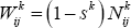 ,
and those with CCP c are given by
,
and those with CCP c are given by 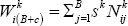 . It is also true that
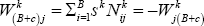 .
.
Scenario 1 assumes that 75 per cent of interest rate derivatives, 50 per cent of credit positions, 20 per cent of commodity positions and 15 per cent of both equity and currency positions are cleared centrally through separate CCP services for each product class. The proportions are similar to the ‘central’ post-reform scenario used in the MAGD exercise for interest rates, credit and currency, but lower for commodity and equity derivatives. The lower penetration of clearing for commodity and equity derivatives acknowledges the slower-than-expected progress towards central clearing of these product classes since the MAGD exercise was undertaken.
| Scenario | CCP service | Per cent centrally cleared, by product class |
|---|---|---|
| 1 | Product specific | 75 per cent interest rate; 50 per cent credit; 20 per cent commodity; 15 per cent equity; 15 per cent currency |
| 2 | Single | As in Scenario 1 |
| 3 | Product specific | 100 per cent of each product class |
| 4 | Single | 100 per cent of each product class |
Scenario 2 assumes that the same proportions of each product class are cleared centrally,
but that this is done through a single CCP service. In this case, 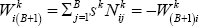 .
.
To provide an upper bound, and to isolate the stability implications of CCP clearing, we also consider a scenario that assumes sk is 1; i.e. all bilateral trades are centrally cleared. We consider the case of separate CCPs – or segregated services – for each product (Scenario 3), as well as a single CCP or fully integrated services for the five products (Scenario 4).
3.3 Expected Exposures and Collateral Demand
The focus of our analysis is future exposures. It is already common practice for variation margin to be exchanged, not only on centrally cleared OTC derivative positions, but also on non-centrally cleared positions – at least for transactions between large banks (ISDA 2014). Accordingly, for the purposes of our analysis, the starting assumption is that all current exposures arising from observed price changes are already fully collateralised by the exchange of variation margin.[6]
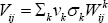
Participant j's expected future exposure to participant i (either
a bank or a CCP) is the expected value of j's losses in the event
of i's default, after accounting for initial margin. This can
be written as
 ,
where:
,
where:
- Vij is equivalent to the variation margin that would have been paid
by participant i to participant j, had participant i
not defaulted. If we define Δpk as the change in
the price of product k since the last variation margin payment (assumed
to be normally distributed around zero), then the next variation margin payment
is given by
 , with
  denotes that participant
j expects to receive a variation margin payment from participant
i, while Vij < 0 denotes that participant
j is expected to pay variation margin to participant i.
For participants i and j, the random variable for variation
margin obligations over the margining period is
denotes that participant
j expects to receive a variation margin payment from participant
i, while Vij < 0 denotes that participant
j is expected to pay variation margin to participant i.
For participants i and j, the random variable for variation
margin obligations over the margining period is  , where
  and
and  , for a 1 × 5
vector
, for a 1 × 5
vector  ,
and a 5 × 5 covariance matrix Ω for price changes
across the five derivative product
classes.[7]
,
and a 5 × 5 covariance matrix Ω for price changes
across the five derivative product
classes.[7]
- Cij is the collateral posted by participant i as initial margin against its derivative positions with participant j. Initial margin is calculated to cover with a high probability any variation margin that participant j would fail to receive in the event of the default of participant i, between the time of default and the time of closeout of the outstanding derivative exposure.[8] We scale up daily derivative price volatilities to cover closeout periods of five and ten days. Five days is the typical closeout period assumed in practice by CCPs to calibrate initial margin on OTC derivative products. The future regulatory minimum in non-centrally cleared settings is ten days, reflecting the likelihood that it will be more difficult to close out positions in a decentralised setting than via a CCP's coordinated default management process. Assuming that the distribution of expected price changes for a given product has a mean of zero, collateral to cover initial margin is calculated as Cij = mσwij Wij, where: m is the number of standard deviations of the portfolio variance covered; σwij is the per-unit portfolio standard deviation; and Wij is the size of the portfolio position.[9] The portfolio standard deviation is, in turn, a function of the price volatility for each product class, which we take from the MAGD exercise (Table 2). The covariance between price changes across products is assumed to be zero. Note that in the case of product-specific CCPs, the price volatility of the portfolio is equivalent to the price volatility of the relevant product class.
| Product class | Daily volatility | 5-day volatility | 10-day volatility |
|---|---|---|---|
| Interest rates | 0.068 | 0.152 | 0.215 |
| Credit | 0.119 | 0.266 | 0.376 |
| Equity | 0.635 | 1.420 | 2.008 |
| Currency | 0.068 | 0.152 | 0.215 |
| Commodity | 0.387 | 0.865 | 1.224 |
| Note: Derivative price volatilities over closeout periods of longer than a day are estimated by multiplying the daily volatility by the square root of the number of days in the closeout period | |||
As an indication of the magnitude of exposure if no initial margin was collected (m = 0 with Cij = 0 for all i and j), Table 3 presents uncollateralised expected exposure over various margining periods. Several observations can be made.
First, exposures increase at a decreasing rate as the assumed time between default and closeout increases. This is as would be expected, given the assumption that prices move in a random walk. Also, as expected, exposures decrease as netting opportunities increase. Clearing all OTC derivative products through a single CCP service lowers exposures relative to the case of using separate CCP services for each product (Scenarios 2 and 4, relative to Scenarios 1 and 3, respectively). Centrally clearing a larger share (Scenarios 3 and 4, relative to Scenarios 1 and 2) of the OTC derivative portfolio also lowers exposures.
| Scenario | 1-day | 5-day | 10-day |
|---|---|---|---|
| 1 | 64.13 | 128.65 | 176.99 |
| 2 | 60.35 | 123.74 | 171.25 |
| 3 | 38.89 | 50.43 | 59.09 |
| 4 | 25.78 | 33.43 | 39.17 |
The collateral required for initial margin assuming 99 per cent coverage of one-tailed price movements (m = 2.33), the minimum coverage level in the PFMIs and the BCBS-IOSCO margining standards for non-centrally cleared derivatives, is presented in Table 4.
| Scenario | Total | Bank-to-bank | Bank-to-CCP | CCP-to-bank |
|---|---|---|---|---|
| 1 | 942.10 | 892.88 | 49.22 | 0.00 |
| 2 | 930.25 | 892.88 | 37.37 | 0.00 |
| 3 | 121.82 | 0.00 | 121.82 | 0.00 |
| 4 | 80.76 | 0.00 | 80.76 | 0.00 |
| Note: A 10-day closeout period is assumed for bank-to-bank margin, a 5-day closeout period is assumed for bank-to-CCP margin | ||||
Each participant holds initial margin against one direction of possible price movements. For either counterparty to a derivative position, uncovered price movements correspond to a single tail of the price-movement distribution, because a counterparty default only gives rise to a replacement cost loss if the default coincides with an adverse price movement. If the default coincides with a favourable price movement, there is no loss. Note that banks post margin against outstanding positions with CCPs, but that CCPs do not post margin with banks. Initial margin again increases with the assumed closeout period, and decreases as the scope for netting increases. In the case of a single CCP, the decline in initial margin requirements is substantial.
When the level of initial margin coverage is high, the remaining uncollateralised exposure is substantially reduced. In interpreting Table 5, it is important to note that the data reflect only the expected uncollateralised exposure that would crystallise in the event of a counterparty default and take no account of the probability of default. Given that CCPs are highly regulated, single-purpose institutions that have a specialist risk management function, the likelihood that a bank's exposure to a CCP crystallises is very low – even though the loss given default is sizeable. This observation will be examined further in Sections 4 and 5.
| Scenario | Total | Bank-to-bank | Bank-to-CCP | CCP-to-bank |
|---|---|---|---|---|
| 1 | 13.86 | 1.30 | 11.94 | 0.62 |
| 2 | 10.84 | 1.30 | 9.06 | 0.47 |
| 3 | 31.09 | 0.00 | 29.54 | 1.05 |
| 4 | 20.61 | 0.00 | 19.58 | 1.03 |
| Note: A 10-day closeout period is assumed for bank-to-bank margin, a 5-day closeout period is assumed for bank-to-CCP margin | ||||
3.4 Realised Exposures
For stability analysis, the tail of the distribution is more relevant than expected outcomes. In the analysis in Sections 4 and 5, therefore, we consider single extreme realisations of OTC derivative price changes and associated ex post exposures.
For each of the five products, let  be the net open position between i and j in product k
and let σk be the standard deviation in the size
of the price changes of product k. Then let vk
be the realised price change in product k in numbers of standard deviations.
The variation margin flows from i to j will be:
be the net open position between i and j in product k
and let σk be the standard deviation in the size
of the price changes of product k. Then let vk
be the realised price change in product k in numbers of standard deviations.
The variation margin flows from i to j will be:
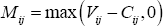
Realised exposures are now defined as any net variation margin receipt that exceeds the size of the initial margin set aside for that position. The realised exposure of participant j to participant i will equal the positive variation margin obligation from participant i to participant j, less the initial margin on the position. We denote this as Mij:
In what follows we consider an ‘expected tail realisation’, which is the expected price change conditional on that price change being larger than the price change on which initial margin was calibrated. This ‘conditional expected future exposure’ is one way to define a ‘large’ price change that isn't simply an arbitrary large number of standard deviations. Of course, since these calculations are based on a normal distribution, the expected tail realisation is only a fraction of a standard deviation above the point at which initial margin is set. Accordingly, in the analysis that follows in Section 4, we supplement this approach with additional tests that consider market outcomes further into the tail.[10]
Initial margin is set on the basis of m standard deviations, which corresponds to a realised price change
of 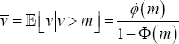 .
For example, a one-tailed coverage level of 99 per cent would have a value
of m of approximately 2.33 and a value of
.
For example, a one-tailed coverage level of 99 per cent would have a value
of m of approximately 2.33 and a value of  of approximately 2.67.
In this case, the ‘realised exposure’ for a single-product portfolio
would be about 0.34 times the portfolio standard deviation (over the exposure
period). A one-tailed coverage level of 50 per cent would have a value of of approximately
0.40.[11]
of approximately 2.67.
In this case, the ‘realised exposure’ for a single-product portfolio
would be about 0.34 times the portfolio standard deviation (over the exposure
period). A one-tailed coverage level of 50 per cent would have a value of of approximately
0.40.[11]
A price change of + standard deviations would represent a large positive price change (to the benefit
of banks with net long positions and to the cost of banks with net short positions),
and a price change of − standard deviations would represent a large
negative price change (to the benefit of banks with net short positions, and
to the cost of banks with net long positions). For a positive  , which represents i
being short and j being long, this upward movement in prices results
in a variation margin payment from i to
j.[12]
, which represents i
being short and j being long, this upward movement in prices results
in a variation margin payment from i to
j.[12]
As an illustration of the magnitudes involved, Table 6 presents realised exposures based on the conditional expectation of a price movement that is beyond the 99th percentile of the price distribution (for an illustrative combination of positive and negative price changes across the product classes).
| Scenario | Total | Bank-to-bank | Bank-to-CCP | CCP-to-bank |
|---|---|---|---|---|
| 1 | 148.52 | 93.38 | 39.87 | 15.26 |
| 2 | 132.83 | 93.38 | 28.18 | 11.27 |
| 3 | 136.46 | 0.00 | 98.69 | 37.78 |
| 4 | 76.64 | 0.00 | 53.28 | 23.36 |
| Notes: Based on the conditional expectation beyond 99 per cent initial margin coverage; assumes price changes of 2.67 standard deviations: positive for interest rates, currency and credit; negative for equities and commodities | ||||
Footnotes
This exercise can also be done using the ratios of net notional assets to gross market value assets with the columns of the matrices. There is little difference in the resulting bilateral net notional positions. [5]
Note that, since variation margin is typically exchanged in cash, these funds may be re-used immediately by the recipient. In contrast, initial margin posted to CCPs is segregated and not available for re-use unless there is a default event. Similarly, under the soon-to-be-implemented BCBS-IOSCO standards, initial margin for non-centrally cleared trades must be held in such a way as to protect the collateral receiver and there are significant limitations on re-use of initial margin. [6]
The zero mean implies that derivatives are fairly priced, valued at zero at the time they are written, with a symmetric distribution of potential price movements such that both long and short sides of the position are as likely to pay as to receive variation margin. [7]
Collateral posted by a bank to a CCP as initial margin is intended to cover any variation margin that the CCP would fail to receive in the event that the bank defaulted, since the CCP retains an obligation to pay variation margin to non-defaulted banks with mark-to-market gains. [8]
Therefore, for standard normal random variable v:  where ϕ(·) is the
standard normal probability density function. This gives
Rij = σwijWij(ϕ(m)
+ m(Φ(m)−1)) where Φ(·) is
the standard normal cumulative density function.
[9]
where ϕ(·) is the
standard normal probability density function. This gives
Rij = σwijWij(ϕ(m)
+ m(Φ(m)−1)) where Φ(·) is
the standard normal cumulative density function.
[9]
An alternative approach, which we leave to future research, would be to use price change distributions that exhibit ‘fat tails’. Such distributional assumptions are common in the finance literature. [10]
Zero initial margin would correspond to a coverage level of 50 per cent, because
for either participant, one half of the price-movement distribution represents
favourable price movements that would not give rise to any replacement cost
loss in the event of counterparty default. With no initial margin held, possible
counterparty losses follow a mixture distribution, with a 50 per cent probability
of being zero, and a 50 per cent probability of following a half-normal distribution
with expected value of  .
Accordingly, expected counterparty losses where zero initial margin is held
would be
.
Accordingly, expected counterparty losses where zero initial margin is held
would be  times the portfolio standard deviation.
[11]
times the portfolio standard deviation.
[11]
It should be noted that, to the extent that our estimates of net open interest are derived from current exposures arising from an unknown price history, the correspondence between signs and directions is essentially arbitrary; we can determine whether positions are directional and whether they are offsetting, but cannot determine whether directional positions are long or short. [12]