RDP 2013-14: Reserves of Natural Resources in a Small Open Economy 2. Motivation

2.1 Theoretical

One approach used to study the effects of a resource price shock is to integrate a natural resource sector within a small open economy DSGE model. A common assumption used in existing literature is that the domestic economy's stock of resource reserves is held constant (or is exogenous with respect to resource prices and their effects on the domestic economy). When choosing to extract resources, firms do not account for the fact that extracting resources today reduces the amount of resources available for future extraction (depletion). In addition, firms are unable to invest in a technology that changes the level of available reserves, for example through exploration and the discovery of new reserves.

Examples of the ‘exogenous reserves’ approach to modelling the natural resource sector include Dib (2008), Garcia and González (2010), Bems and de Carvalho Filho (2011), Bodenstein, Erceg and Guerrieri (2011), Lama and Medina (2012) and Natal (2012). Similar abstractions are also common in DSGE models developed by central banks, including Australia (Jääskelä and Nimark 2008), Canada (Murchison and Rennison 2006), New Zealand (Lees 2009) and Spain (Andreás, Burriel and Estrada 2006).

Although a useful simplifying assumption for some purposes, a limitation of the ‘exogenous reserves’ approach is that there is nothing inherently natural resource-like in the behaviour of resource producers. This raises some important questions: to what extent does the assumption of exogenous reserves matter for understanding the propagation of resource price shocks? Would the responses look especially different if one allows for endogenous reserves due to exploration and depletion? We attempt to address these questions with specific reference to the effects of a resource price shock in a small open economy model.

In terms of related literature, the only paper that we are aware off that nests an endogenous reserves structure in a DSGE model is Veroude (2012) who studies business cycle correlations for Australia using a closed economy real business cycle model. Our work complements this research by studying the open economy implications of endogenous reserves with specific reference to the effects of shocks to international resource prices. We believe that openness is an important consideration because much of the resource sector's output and capital formation is exported and imported respectively, and this has implications for relative prices and the real exchange rate.

There is a separate and quite extensive literature on the optimal extraction of natural resources and investment and exploration decisions, but not within the context of a small open economy. A non-exhaustive list of useful references includes Pindyck (1978), Reiss (1990), Heal (1993), Sweeney (1993) and Bohn and Deacon (2000). There is also very informative literature studying the comparative statics of general equilibrium models with multiple sectors including resources (see, for example, Gregory (1976) and Corden (2012)), although these models do not incorporate expectations or dynamics.

2.2 Empirical

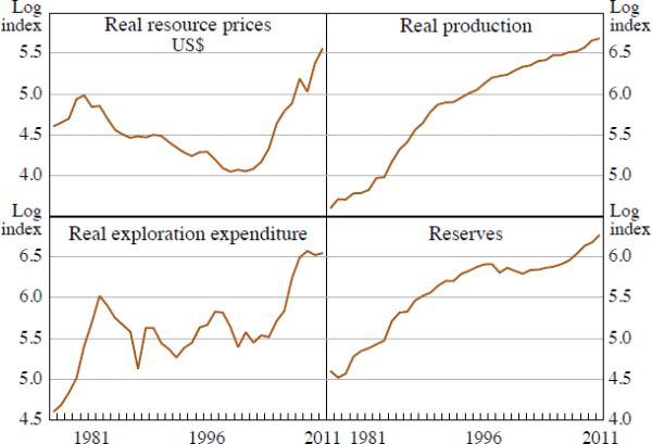
Figure 1 highlights some of the key developments in the Australian resource sector since 1976. Figure 1 shows measures of average prices, average production (extraction), real exploration expenditure, and the average stock of reserves in the sector.^[2] Reserves for each resource commodity are measured to include both economically demonstrated reserves – reserves considered to be economically profitable for extraction purposes – and sub-economic reserves, which are not considered to be currently viable but that may become viable in the future with higher resource prices or an advance in technology that reduces costs.^[3] The resources included in these measures are iron ore, coal, oil and petroleum (including crude oil, condensate and liquefied petroleum gas (LPG)), natural gas, five base metal ores (bauxite, copper, lead, nickel and zinc), and gold. Together these resources accounted for approximately 88 per cent of Australia's total resource exports, and 66 per cent of total goods exports in 2011/12.

Summarising the main stylised facts:

1. Real resource prices trended down for much of the sample but then increased around the turn of the millennium reflecting strong commodity demand, particularly from China.
2. Production growth was most rapid in the mid to late 1980s but has since stabilised.^[4]
3. Real exploration initially peaked in the early 1980's and then declined for much of the period in which real resource prices fell. From around the mid 2000s, real exploration activity began to grow rapidly as the increase in resource prices became sustained.
4. The pace of growth in reserves generally slowed over the 20 years between 1980 and 2000 and accelerated from the mid 2000s. This suggests that at least some of the pick up in exploration has resulted in the discovery of new reserves.

To provide insight into the broader effects of a resource price shock on the Australian economy, we use a simple structural vector autoregression (VAR) with annual data. We identify the effect of a shock to resource prices using the assumption that resource prices are contemporaneously uncorrelated with domestic variables and the real exchange rate. That is, we estimate:^[5]

where z_t is vector of observable variables including real resource prices, the real TWI, the ratio of non-mining GDP to the stock of natural reserves, the ratio of resource sector capital expenditure to the stock of natural reserves, and inflation (in that order),^[6] and A₀ is a matrix with ones along its main diagonal and zeros in the off-diagonal elements in its first row. The latter reflects the identifying assumption that resource prices are contemporaneously uncorrelated with the remaining variables in the VAR.

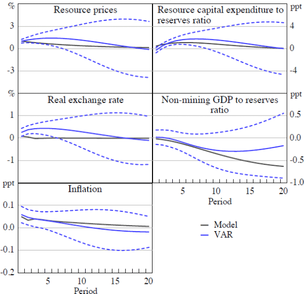
Figure 2 reports the impulse response functions (IRFs) due to a 1 per cent exogenous increase in resource prices. Each IRF is measured in terms of the percentage deviation from its sample mean (or percentage point deviation where appropriate), and we report the 95 per cent (asymptotic) confidence intervals. In addition to the VAR IRFs, we also report the IRFs from our theoretical model in general equilibrium with endogenous reserves. The latter are produced from a theoretical model in which we estimate a subset of the model's parameters using a Generalised Method of Moments (GMM) estimator, and the remaining parameters are calibrated (Section 4.2 provides further details).

The results in Figure 2 suggest that resource price shocks are very persistent and have significant effects on both the resource sector and the broader economy. In particular, the VAR IRFs imply that an exogenous 1 per cent increase in resource prices leads to a persistent real appreciation of the exchange rate, a temporary increase in inflation and an increase in resource capital expenditure relative to reserves. A small, though not statistically significant, decline in the ratio of non-mining GDP to reserves is also observed.

Interestingly, our theoretical model is able to reproduce these results quite well in terms of the sign, amplitude and persistence of the IRFs. The main exception is the real exchange rate. Although our model is able to reproduce an appreciation, it is neither sufficiently large nor persistent when compared with the response identified in the VAR. Nevertheless, in view of the theoretical model's overall ability to match the VAR IRFs, we use these GMM estimates to help parameterise both the partial and general equilibrium models discussed below.

Footnotes

All averages – prices, production and reserves – are export-weighted geometric averages, where the export weights used are fixed at the sample averages for 1976 to 2011. [2]

See Geoscience Australia (2012) for further discussion on the classification of reserves. Prior to 1992, all reserve measures are based on economically demonstrated reserves only and are spliced to the post-1992 series. Estimates for production and reserves in 2011 are inferred using the growth rates implied in Australian Bureau of Statistics (ABS) data (ABS Catalogue No 5204.0). [3]

However, the recent high levels of investment in the mining sector are forecast to increase production over the medium term, see Bureau of Resources and Energy Economics (2013). [4]

A deterministic time trend and constant are also included in each regression. It should be noted that similar estimates are obtained using HP-filtered data or differenced data. [5]

For a full description of the data used, see Appendix A. [6]