RDP 2013-13: Inventory Investment in Australia and the Global Financial Crisis 5. Econometric Analysis
November 2013 – ISSN 1320-7229 (Print), ISSN 1448-5109 (Online)
- Download the Paper 839KB
5.1 Basic Framework
Firm-level data provide a quasi-experiment to determine the role of credit constraints in inventory investment. To understand the setup of the model, consider the following hypothetical example.
Suppose there is an experiment in which firms are randomly selected from the population of Australian businesses. During the experiment, the firms undertake their daily business of producing output, paying workers and investing in inventories. Furthermore, as part of their regular business operations, all the firms in the experiment must, at some point, take out a bank loan to invest in new stocks and maintain production. The firms are randomly allocated to either a control group or a treatment group. The experiment is deliberately designed so that the only difference between the two groups is that firms in the treatment group are rejected by the bank for a loan, whereas firms in the control group obtain the loan. Therefore, loan rejection acts as the ‘treatment’ in this experiment.
The inventory investment behaviour of the two groups of firms is observed, both before and after the firms apply for the bank loan. If the rejected firms are observed to reduce their investment spending relative to the accepted firms after applying for a loan, then it would be safe to conclude that, due to the random assignment of firms, the fall in inventory investment was caused by the inability to get a loan. In other words, this experiment would provide strong evidence that firms’ inventory investment is affected by constraints on the availability of bank credit.
In reality, it is not possible to conduct such an experiment. But it is possible to exploit a ‘quasi experiment’ which closely replicates the conditions of the laboratory in a real-world setting. I identify the effect of credit conditions on inventory investment using the variation in the maturity structure of the debt owed by Australian firms in the period before the global financial crisis. In particular, I separate listed companies into two groups; companies that were ‘unlucky’ to have a debt maturity structure such that a large share of their outstanding debt fell due at the peak of the crisis in 2008/09 and companies that were ‘lucky’ in that most of their debt fell due at some other (non-crisis) time.
The logic is that the unlucky firms would have been forced either to repay or refinance a higher proportion of their debt at a time when lenders were concerned about heightened credit risk, and hence looking to scale back the supply of credit. In this experiment, the unlucky firms are the treatment group and the lucky firms are the control group. If the unlucky firms reduced their inventory investment by more than the lucky firms during the crisis, then, all other things being equal, this would provide evidence that credit constraints significantly affected inventory investment. A similar methodology is used by Almeida et al (2009) to identify the effect of debt maturity on corporate fixed capital investment in the United States.
To understand the regression framework it helps to outline the steps that are required to get to the estimating equation. The model in levels is:
where the dependent variable is the (log) stock of inventories of firm i that operates in industry j in year t (Iijt).
The explanatory variables include a dummy variable for whether the period is
prior to the 2008/09 crisis (t = 0) or during the crisis (t
= 1) (CRISISt) and a dummy variable for whether the share
of outstanding debt of firm i in the pre-crisis period that is due
within one year exceeds 80 per cent (STDEBTi), as well
as the interaction between both dummy variables ( ).
The reason for choosing a cut-off level for the short-term debt ratio of 80
per cent is discussed below.
The specification also includes a set of firm-level controls that vary over time (Xijt), such as the size and profitability of the firm. The equation also includes a firm-level fixed effect (θi), which is designed to capture all unobservable firm characteristics that influence the average level of inventory holdings, and an industry-year fixed effect (λjt), which captures unobservable industry-level shocks to inventory investment that vary over time.
Before estimation, I collapse the data so that there are just two periods – the pre-crisis and crisis periods. I define the pre-treatment period to be 2007/08 and the post-treatment period to be 2008/09. I next transform each variable by taking the difference over time between the pre-crisis and crisis periods to obtain the following equation to be estimated:[7]
where the dependent variable is the change in the (log) stock of inventories of firm i during the crisis (ΔIij) and the key explanatory variable is the dummy variable for whether the share of outstanding short-term debt of firm i exceeds 80 per cent (STDEBTi). Equation (2) is known as a difference-in-differences model. The main coefficient of interest is δ in Equation (2), which is the difference-in-differences estimator. Note that, by estimating the equation in first differences, I effectively eliminate the firm-level fixed effect. So this specification controls for factors that affect inventory investment and that vary across firms but are unobservable and do not vary with time.[8] Moreover, the specification includes an industry-level fixed effect, which implies that I identify the relationship between the shock to credit conditions and inventory investment through variation within each industry.
5.2 Data
The data underpinning the regression analysis are derived from the semi-annual financial reports of listed Australian companies provided by Morningstar. The sample includes 276 firms listed on the Australian stock exchange that operate in one of three sectors: industrials, consumer staples or consumer discretionary.[9] The original sample period covers from 1989/90 to 2011/12, although the regressions are only estimated on data from 2007/08 and 2008/09.
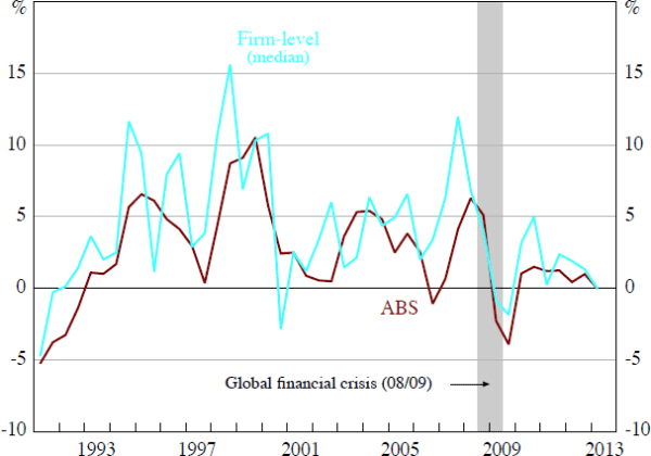
The (real) annual growth rate of inventories acts as the dependent variable in the regression model. In the semi-annual reports, each company reports the book value of the stock of inventories. As inventory investment is very short-term in nature, the book value is likely to be a good approximation for the market value of the stocks. There is a reasonable correlation between the growth in inventories reported in the national accounts and that based on the measure of inventory investment constructed on the basis of the company reports data (Figure 9). This suggests that any findings based on the firm-level data are likely to have a direct bearing on the aggregate economy.

Sources: ABS; Morningstar; author's calculations
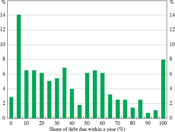
The key explanatory variable in the model is a firm-level dummy variable indicating whether the share of total debt due within one year in the pre-crisis period is greater than 80 per cent or not. The results are not sensitive to this cut-off level; I obtain similar results if the cut-off is defined at either 70 per cent or 90 per cent. Looking at the cross-section in 2007/08, Australian companies generally either held very little short-term debt (as a share of total debt) or they held a lot of short-term debt in 2007/08 (Figure 10). The clear divide between firms with relatively high and low shares of short-term debt supports the identification strategy to split firms into ‘lucky’ and ‘unlucky’ groups.

Sources: Morningstar; author's calculations
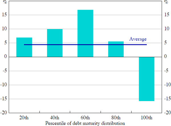
The underlying firm-level data also indicate that firms with a relatively high share of debt due within a year (the top quintile of the debt maturity distribution) were much more likely to scale down inventories than firms with a relatively low share of short-term debt falling due (Figure 11).[10]

Note: Difference in the (log level of) inventories between 2007/08 and 2008/09
Sources: Morningstar; author's calculations
5.3 Covariate Matching
To establish a causal effect of short-term debt on inventory investment, ideally the firms would be randomly assigned to the treatment and control groups. Otherwise, any differences in investment behaviour between the two groups during the crisis could be due to confounding factors, such as unobservable differences in business models and riskiness.
To address this issue I estimate the model using ‘covariate matching’. Specifically, each treated firm is ‘paired’ with the untreated firm that is most similar in terms of observable characteristics. There is a range of available matching estimators; I use the Abadie and Imbens (2011) matching estimator. This estimator minimises the difference between a vector of observed covariates across treated and untreated firms, finding controls based on matches for which the difference between the vectors is smallest. Matching on covariates, by definition, removes any differences between the treatment and control firms and hence eliminates any bias in estimating causal (or ‘treatment’) effects. But when there are many covariates, it is not practical to match directly on all covariates, particularly when the variables are continuous. Instead, the multiple covariates generally need to be summarised by a scalar through some metric, which measures the closeness of two observations.[11] The estimator allows those firms chosen as controls to serve as matches more than once.[12] I select one matched control firm for each treated firm (although more firms could be chosen).
The vector of matching variables includes the pre-crisis levels of real inventories and real sales for each firm. The inclusion of lagged inventory and sales terms arises from a target adjustment motive; firms are assumed to want to lower inventories when the inventory-to-sales ratio is high, so there should be a negative coefficient on the lagged level of inventories and a positive coefficient on the lagged level of sales. The real annual growth rate of sales is also included to control for firms’ expectations of demand. The effect of higher expected sales growth is somewhat indeterminate; if inventories are primarily used to smooth production then the coefficient should be negative, but if inventories serve mainly to avoid running out of stocks then the coefficient should be positive.
The matching procedure also includes controls for firm size (the log level of assets) and leverage (the debt-to-assets ratio), as well as indicators that capture a firm's ability to offset external financing shocks, such as its level of liquid asset holdings (the cash-to-assets ratio) and its use of trade credit (the trade credit-to-assets ratio). More detailed information on the construction of each variable is included in Appendix A. The estimator produces exact matches on categorical variables (e.g. industry classification), but only imperfect matches on continuous variables (e.g. size) so an adjustment is made to correct for such a bias. In addition, the estimator produces standard errors that are robust to heteroscedasticity.
As an example of the matching procedure, two of the listed motor vehicle dealers – Automotive Holdings Group and the Adtrans Group – are classified as treated companies because they had short-term debt ratios exceeding 80 per cent (83.5 per cent and 85 per cent respectively). The matching procedure estimates that, for both treated companies, the best matched control is the other listed motor vehicle dealer – A.P. Eagers – which had a short-term debt ratio less than 80 per cent (58.7 per cent). This matching makes sense given the firms are in the same industry and operate with similar business models.
Summary statistics for the key variables across the treatment and matched control groups are shown in Table 1 below.
| Variable |
Mean | Median | Std dev | |||||
|---|---|---|---|---|---|---|---|---|
| Treated | Control | Treated | Control | Treated | Control | |||
| Pre-crisis, 2007/08 | ||||||||
| Assets (log level) | 4.2 | 4.2 | 4.2 | 4.0 | 1.7 | 1.5 | ||
| Cash-to-assets ratio (%) | 8.7 | 8.6 | 5.0 | 6.0 | 9.5 | 9.3 | ||
| Trade credit-to-assets ratio (%) | 39.8 | 41.0 | 40.2 | 37.1 | 20.5 | 21.2 | ||
| Debt-to-assets ratio (%) | 25.7 | 23.7 | 24.3 | 23.9 | 19.1 | 13.3 | ||
| Cash flow-to-assets ratio (%) | 0.9 | 3.6 | 2.4 | 5.6 | 11.2 | 10.1 | ||
| Post-crisis, 2008/09 | ||||||||
| Real inventories (% change) | −23.5 | −10.1 | −9.0 | −3.2 | 57.3 | 44.7 | ||
| Real sales (% change) | 0.0 | −6.8 | −4.0 | −3.8 | 57.3 | 43.4 | ||
|
Sources: Morningstar; author's calculations |
||||||||
As the summary statistics indicate, the treated and control firms are very similar in all relevant characteristics. In terms of the control variables, the main notable difference between the two types of firms is that the control firms are more profitable than the treated firms, as shown by the higher cash-flow-to-assets ratio.
5.4 Parallel Trends Assumption
The key assumption of the difference-in-differences modelling strategy is that the inventory investment behaviour of the treated and control firms would have followed the same trend had the 2008/09 crisis not occurred (i.e. in the absence of treatment). This is known as the ‘parallel trends’ or ‘common trends’ assumption.[13]
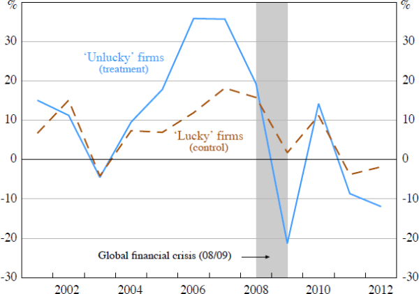
To see if this assumption is justified, it is instructive to consider how inventory investment of the treated firms evolved before and after the crisis relative to that of the control firms (Figure 12). Overall, inventory investment follows a similar cyclical pattern for both groups. Inventory investment clearly fell more sharply for the treated firms than for the control firms during the crisis period, which is consistent with the hypothesis that binding short-term credit constraints caused investment to fall. However, there is also some evidence that investment diverged in the period just prior to the crisis, with inventories growing more rapidly for the treated firms. While this pre-crisis divergence raises some doubts about the validity of the parallel trends assumption, it appears that, overall, the graphical analysis supports the proposed identification strategy.

Notes: Treatment group includes firms with a short-term debt ratio greater than 80 per cent in 2007/08; control group includes firms that are matched to the treatment group based on covariates
Sources: Morningstar; author's calculations
Footnotes
To account for differences in reporting seasons across firms, I calculate the pre-treatment level of inventories by taking the average of the stock levels reported at the ends of December 2007 and June 2008. Similarly, I calculate the post-treatment level of inventories by taking the average of the stock levels reported at the ends of December 2008 and June 2009. I then calculate inventory investment as the difference between these two estimates. For the reported share of short-term debt, I calculate the average share of short-term debt outstanding reported at the ends of December 2007 and June 2008. [7]
The specification will control for certain characteristics of the products typically sold by each firm. For example, food manufacturers typically produce goods that are perishable and hence have a short shelf life. These firms will typically hold relatively low levels of stocks, on average. [8]
According to the Global Industry Classification Standard (GICS), the consumer staples sector comprises manufacturers and distributors of food, beverages and tobacco as well as producers of non-durable household goods and personal products. It also includes food and drug retailing companies as well as supermarkets and department stores. The consumer discretionary sector includes manufacturers of motor vehicles, household durable goods, clothing, textiles and leisure equipment. It also includes services companies that cover hotels, restaurants and other leisure facilities, media production and services, and consumer retailing and services. The industrials sector includes manufacturers of capital goods (e.g. machinery and electrical equipment), companies that provide transportation services (e.g. airlines) and companies that provide commercial services and supplies (e.g. employment services). These sectors were chosen to reflect the goods distribution sector (i.e. retail trade, wholesale trade and manufacturing). [9]
To minimise the impact of outliers, I ‘winsorise’ all the variables used in the regression analysis at the bottom and top 1 per cent of their respective distributions. Winsorising involves replacing extreme values with certain percentiles. So, for example, if the top 1 per cent of a distribution is winsorised, any value beyond the 99th percentile is replaced by the value at the 99th percentile. The main results in the paper are little affected by this procedure. [10]
The Abadie and Imbens (2011) estimator matches observations in the treatment and control groups based on the Mahalanobis distance. The Mahalanobis distance is a descriptive statistic that provides a relative measure of a data point's distance from a common point. It is different to Euclidean distance because it accounts for correlations in the dataset and is scale-invariant. [11]
This lowers the estimation bias (but increases the variance) compared to matching without replacement. [12]
The identifying assumption does not require that the level of investment is the same for the two groups, as such differences are eliminated in estimation. [13]

