RDP 2013-08: International Business Cycles with Complete Markets Appendix B: Solving the Model

B.1 The Optimality Conditions

An equilibrium allocation in this economy can be computed as the solution to a social planner's problem. Taking the initial conditions as given, the planner chooses state-contingent plans for each agent j ϵ J = {1,2} to maximise the expected discounted sum of their weighted utilities

subject to the law of motion for capital

the law of motion for habits

as well as the global resource constraint

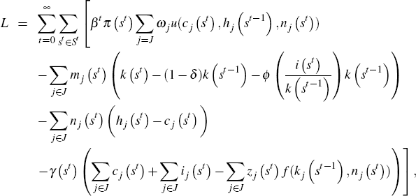
The Lagrangian associated with the planner's problem is given by

where and are the state-contingent paths of Lagrange multipliers associated with constraints in Equations (B2), (B3), and (B4). Equating the gradient of the Lagrangian to zero we obtain

where u₁ (·) is the partial derivative of u with respect to its first argument. We use the same notation to denote the other partial derivatives.

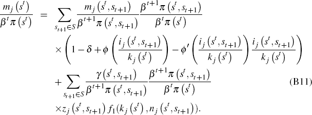
The intertemporal conditions given by Equations (B8) and (B9) can be rearranged as

and

By denoting , and we can rewrite Equations (B10) and (B11) as

and

In a similar way, Equations (B5) and (B7) can be rewritten as

and

Let Λ_j (s^t) denote the marginal utility of consumption of agent j after history s^t. Then from Equations (B12) and (B13) it follows that

where π (s_t+1 | s^t) denotes the conditional probability of s_t+1 given s^t, and π (s^t | s^t) = 1.

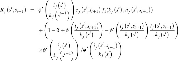
Let R_j (s^t,s_t+1) denote the realised one-period gross rate of return on capital in country j after realisation of history (s^t,s_t+1)

Then the first order conditions can be reformulated as

for j ϵ J.

B.2 Optimality Conditions with the Functional Forms

The instantaneous utility function takes the form

The production function is

The capital adjustment cost function is

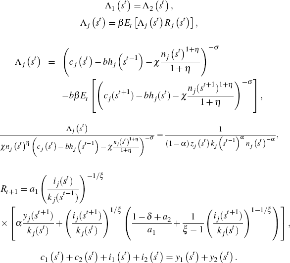
where the restrictions that ϕ′ (δ) = 1 and ϕ (δ) = δ require that a₁ = δ^1/ξ and . Symmetry between the two economies implies that ω₁ = ω₂. Incorporating specific functional forms, the optimality conditions can be rewritten as

B.3 Parameter Values for the Benchmark Model

Productivity follows a process similar to that specified by Kehoe and Perri (2002):

The innovations to the productivity process are zero mean serially independent bivariate normal random variables with the contemporaneous covariance matrix

Standard/estimated values are as follows:

• Capital income share α = 0.36 and coefficient of relative risk aversion σ = 2, as in Kehoe and Perri (2002)
• Elasticity of labour supply 1/η = 1.43, that is, η = 1/1.43 = 0.6993, as in Correia et al (1995)
• Intensity of habits b = 0.73, as in Jermann (1998).

The calibration targets are: n_ss = 1/3;i_ss/y_ss = 0.25;k_ss/y_ss = 10. The calibrated parameters are as follows:

• Depreciation rate: δ = i_ss/k_ss = (i_ss/y_ss)/(k_ss/y_ss) = 0.025
• Discount factor: β = (α (y_ss/k_ss)+1−δ)⁻¹ = (0.36−0.1+1−0.025)⁻¹ = 0.989

• From it follows that

  

  View MathML

• From the labour supply equation in the non-stochastic steady state , it follows that the weight of labour in the utility function χ is:

  

  View MathML

The other steady-state values are as follows:

B.4 The Numerical Procedure

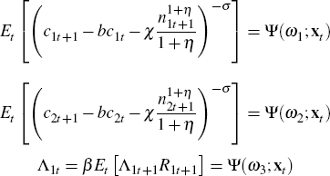
The model is solved using a variant of the ergodic set methods described by Maliar, Maliar and Judd (2011). The algorithm we use is classified by Judd, Maliar and Maliar (2009) as belonging to the stochastic simulation class of methods. The approach is to replace conditional expectations with smooth parametric approximation functions of the current state variables and a vector of parameters, and then iterate on the parameter values until a rational expectations equilibrium is achieved. The four conditional expectations are parameterised as follows

where x_t = [k_1t,k_2t,c_1t−1,c_2t−1,z_1t,z_2t]. From the first order condition for consumption in the home country we have

Re-arranging yields

From the first order condition for labour in the country 1

it follows that

From the risk-sharing condition:

we obtain

and from the country 2 supply equation we get

Current consumption in each country is therefore given by:

Labour in each country is given by

The algorithm is implemented as follows:^[6]

1. Obtain an initial guess for ω = [ω₁,ω₂,ω₃,ω₄]. We obtain the initial guess using the genetic algorithm and then homotopy. Fix k_j0 = k_ss, h_j0 = c_ss and z_j0 = 1 for j ϵ J, and draw a sample of size T of the exogenous stochastic shock .
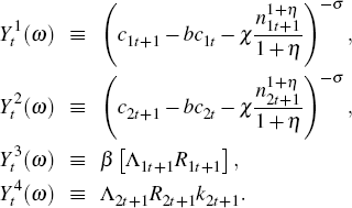
2. Replace the conditional expectations with the parameterised functions Ψ(ω_r;x_t), r = 1…4. Calculate using Equations (B18), (B19), (B20) and (B21), and the law of motion for habits, Equation (B3). Calculate using the production function, the law of motion for capital given in Equation (B2) and the global resource constraint, Equation (B4). Similarly compute .

3. Set

   

   View MathML

   and minimise the sum of squared residuals for the equation where is the regression error. That is, find

   

   View MathML

   where ζ, is the parameter vector to be estimated.

4. Iterating on w_r, find the fixed point . Update w_r using the algorithm given.

Footnote

Further details on this class of algorithm are provided by den Haan and Marcet (1990). For a more formal description and related proofs, see Marcet and Marshall (1994). [6]