RDP 2012-01: Co-movement in Inflation Appendix A: The Panel VAR

A.1 The Model in More Detail^[19]

Consider a dynamic panel data model shown in Equation (A1) where y_i,t represents an observation for cross-section i = 1,…,N in time period t = 1,…,T

If we generalise Equation (A1) and allow y_i,t to be a vector of G variables, denoted in bold as y_i,t, then Equation (A2) below represents a panel VAR model:

Where Y_t represents the NG × 1 vector formed by stacking the vector y_i,t in the cross-sectional dimension, that is, , and are G × NG matrices of coefficients for up to P lags of Y_t to be included in the VAR. Note also that e_i,t is a G × 1 vector of mean zero and iid errors. Finally, denoting D₁,…,D_p as stacked-by-i NG × NG matrices of coefficients, and also allowing for a C × 1 vector of exogenous explanatory variables denoted C_t with coefficient matrix A, then we obtain Equation (A3):

Where E_t is a NG × 1 vector of random disturbances, E_t ~ N(0,Ω).

Define as the vector formed by stacking the P lags of the right-hand-side variables. Now we can write Equation (A3) as a system of the form:

Where in the above equations , δ_i is a (NGP + CP) × 1 vector formed by stacking the rows of D = [D₁,…,D_p,A₀,…,A_p−1] and finally δ is formed by stacking δ_i and is a vector containing all the coefficients of the system.

Equation (A5) describes the factorisation of the coefficients vector as discussed in the main text. We include common, country-specific and variable-specific factors, alongside the exogenous variables as key drivers of the data. In Equation (A5), the dimension of is 38 × 1, much smaller than the total number of coefficients in the unrestricted model and making estimation feasible using a realistic sample size. The 's represent matrices of appropriate dimensions made up of 1's and 0's and are designed to pick out the relevant coefficients relating to our factorisation. The error term captures un-modelled features of δ and throughout we assume that V = σ²I_NGP+CP.^[20]

Finally, substituting Equation (A5) into Equation (A4), we get:

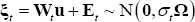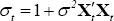Where and and the error term where .^[21]

A.2 Estimating the Model

Bayesian methods were used to estimate the panel VAR. Equation (A7) represents the seemingly unrelated regression (SUR) form of the model:

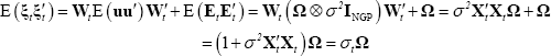
Where and . It should be clear that for σ² > 0 the error term implied by the model is heteroskedastic, where .^[22] While in the baseline estimation we set σ² = 0, it is also possible to treat σ² as a parameter to be estimated.

We employ a semi-conjugate prior for the parameters θ, σ² and Ω:

Where .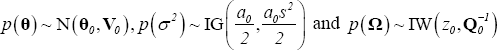

When estimating the model over the full sample of data from 1981:Q2 to 2011:Q1 an uninformative prior was used. When estimating the model over the ‘low-inflation’ sample a training sample from 1981:Q2 to 1991:Q2 was used to initialise the prior. Specifically, the prior mean for the coefficients vector was set equal to the OLS estimate of the SUR model using the training sample, with a prior variance equal to the identity matrix. For the inverse Wishart prior for Ω we set z₀ = NG + T₀ (where T₀ = 41 is the size of the training sample) and where is the variance covariance matrix of the residuals in our OLS training sample regression. Finally, in the case where σ² is allowed to be non-zero, for the inverted gamma prior for σ² we set a₀ = 1 and s² equal to the average of NG individual variance estimates obtained from simple AR (2) regressions estimated for each variable. These prior choices largely follow Canova et al (2007).

Information from the data can be summarised by the kernel of the likelihood function for the SUR form of the model:

Combining the prior information with the likelihood does not offer an analytical solution for joint posterior distribution of parameters. Therefore we used Monte Carlo Markov Chain (MCMC) techniques to simulate the posterior distribution. Since analytical expressions for the conditional posterior distributions of θ and Ω do exist given our semi-conjugate choice of prior, we employ the Gibbs sampler. However, the conditional posterior distribution of σ² is non-standard and a Metropolis step is used within the Gibbs loop to obtain the correct posterior distribution. The steps in the estimation process are as follows.

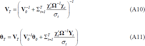
1. Given starting values for σ² and Ω, draw θ from a normal distribution 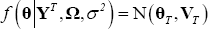with mean and variance given by:

   

   View MathML

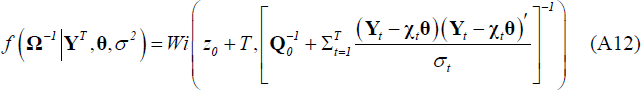
2. Given the starting value for σ² and the draw of θ obtained in Step 1, draw Ω from an inverted Wishart distribution:

   

   View MathML

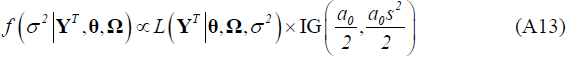
3. Given the draws for θ and Ω obtained in Steps 1 and 2, draw σ² employing a Metropolis step. To do this, we evaluate the kernel of the posterior (Equation (A13) below) at a new candidate draw of σ² relative to the previous draw. The candidate draw is generated from a normal distribution centred at the previous draw, i.e. 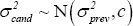where we calibrate the variance c to achieve an acceptance rate of between 30 and 50 per cent. The candidate draw is accepted with a probability equal to the minimum of 1 and the ratio of the kernels.^[23]

   

   View MathML

4. Repeat Steps 1 to 3 conditional on the most recent draw for the parameters.
5. Check for convergence of the posterior distribution after discarding a burn-in sample to remove any influence of the choice of starting values.

We used 20,000 draws in the Gibbs sampler routine described above to estimate the posterior distribution of the parameters, with the first 10,000 draws discarded as a burn-in sample. To check convergence of the posterior distribution the first and second moments of the coefficient estimates at various points of the chain were compared.

Footnotes

The notation in this section largely follows Canova et al (2007). [19]

Canova and Ciccarelli (2009) provide a detailed example of this setup in a simple two-country and two-variable setting. [20]

For σ² > 0 the model implies a specific form of heteroskedasticity in the error term. [21]

To see this, recalling the spherical assumption made about V, then the variance covariance matrix of the error term in Equation (A6) takes the form:

[22]

More details can be found in Canova et al (2007). [23]