RDP 2010-08: Sources of Chinese Demand for Resource Commodities 4. Explaining Chinese Resource Imports
November 2010
- Download the Paper 499KB
To examine global trade in non-oil resource commodities[11] we use the gravity model, which predicts that trade between two countries is positively related to their economic size and negatively related to the cost of transportation (typically proxied by the distance between the two countries' capital cities). We proceed in three stages. First, we estimate a baseline equation explaining bilateral resource imports using an unbalanced panel of 180 economies over the period 1980 to 2008. Second, we adjust the equation to separate out the effects of importing country domestic expenditure, domestic investment and exports on resource imports. We then use a dummy variable to test if – controlling for other determinants of commodity trade – China's imports of resources depend on its (mainly manufacturing) exports, and whether this relationship is different for China than for other resource importers.
4.1 Modelling Trade in Resources – Estimation Strategy
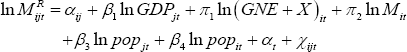
Our data consist of an unbalanced panel of real bilateral non-oil resource imports,
real GDP, real expenditure components of GDP and population for 180 economies
over 1980–2008 (see Appendix E for details). We start by estimating
a baseline gravity model for resource imports. This includes both country-pair
fixed effects and time-fixed effects, and is estimated using ordinary least
squares. The real level of resource imports  by country i from
country j, in year t is expressed as follows:
by country i from
country j, in year t is expressed as follows:

where GDP refers to real gross domestic product, and pop refers to population. Although some authors enter real GDP per capita as a dependent variable rather than including GDP and population separately, it is also common to leave the coefficients on population unconstrained. The time-fixed effect (αt) is a dummy variable for each time period, capturing common global trends, such as macroeconomic shocks and commodity prices. The country-pair fixed effect (αij) captures all factors without time variation that affect the volume of trade between two countries; for example, relative differences in resource endowments and the distance between two countries. Country-pair fixed effects are included because they can eliminate substantial bias in gravity models (Cheng and Wall 2005).[12] To estimate this equation using least squares, we take the log of both sides, resulting in the following specification:

To examine the extent to which – controlling for other factors – commodity imports are correlated with individual components of importing country GDP, such as domestic expenditure on consumption and investment, and exports, we need to include these components in the specification.
We know from the accounting identity that:

where: C, I, G, X and M refer to household consumption, gross capital formation, government consumption, total exports and total imports, and GNE refers to gross national expenditure. Our hypothesis is that a country's resource imports are correlated with a combination of gross national expenditure less imports (hereafter GNE–M) and exports.[13] GDP is an unweighted linear combination (the sum) of these components; however, a priori, the nature of their relationship with resource imports is unknown. While it would be convenient to assume that resource imports were a function of a weighted arithmetic average of GNE–M and X in the importing country, identifying the weights of this average would be problematic in least squares estimation.[14] Assuming that resource imports are correlated with a geometric average of these two variables at least allows the weights to be identified, and allows for the possibility of a nonlinear relationship. Therefore, we also propose the following gravity equation:

We estimate this equation in the log form:
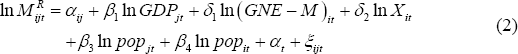
It may seem unusual to include a trade variable on both the right- and left-hand-sides of the estimated equations. But the fact that we are regressing resource imports by country i from country j on country i's total exports to the rest of the world means that endogeneity is unlikely to be a serious problem. As an additional precaution, for each economy we also subtract its imports of resources from total imports. This ensures that the dependent variable is not appearing on both sides of the equation, though for most economies the share of resources in total imports is small. For China, this share was a little more than 2 per cent until 2004, but even today, resources still account for only around 10 per cent of total imports.
We can perform a similar exercise to consider the effect that investment, on its own, has on resource imports, by including GDP less investment (hereafter GDP–I) and investment (I) separately on the right-hand-side of the equation:
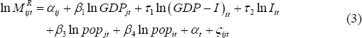
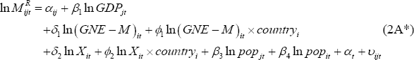
As we are particularly interested in the determinants of China's resources imports, we adjust Equation (1) to examine whether China's imports of commodities are more responsive to its GDP compared to other economies, as follows:
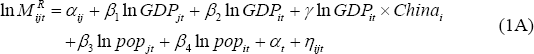
where the variable Chinai is a dummy variable that is equal to one if the importing country is China. Hence, β2 + γ is the total marginal effect of an increase in China's GDP on its resource imports.
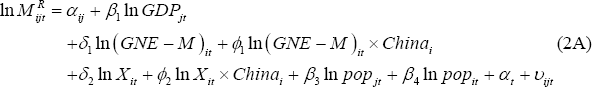
Using this framework we can also ask whether China's commodity imports are more responsive to the ‘domestic’ components of GDP or exports than are the resource imports of other economies:
Finally, we also augment Equation (3) with China dummies, to consider the responsiveness of China's resource imports to investment on its own:

As the gravity model is estimated in log form, the model cannot be estimated for observations with zero trade flows. Thus, all observations without trade are excluded from the regressions.[15] To prevent economies with very little resource trade having an undue influence on the results, we also exclude all observations where real resource imports were particularly small.
4.2 Results
Table 3 presents regression results for resource imports. The three ‘Baseline’ columns present the results for Equations (1) to (3) without China dummies, while the three ‘China effect’ columns report results including China dummies (Equations (1A) to (3A)). While all regressions were estimated with time and country-pair fixed effects, for the sake of brevity these coefficients are not reported.[16]
| Baseline | China effect | ||||||
|---|---|---|---|---|---|---|---|
| (1) | (2) | (3) | (1A) | (2A) | (3A) | ||
| GDPjt | 0.71*** | 0.78*** | 0.72*** | 0.72*** | 0.78*** | 0.73*** | |
| GDPit | 1.67*** | 1.40*** | |||||
| GDPit×Chinai | 0.88*** | ||||||
| Xit | 0.98*** | 0.83*** | |||||
| Xit×Chinai | 0.12 | ||||||
| (GNE–M)it | 0.13*** | 0.08** | |||||
| (GNE–M)it×Chinai | 0.99 | ||||||
| Iit | 0.52*** | 0.46*** | |||||
| Iit×Chinai | 0.51 | ||||||
| (GDP–I)it | 0.98*** | 0.76*** | |||||
| (GDP–I)it×Chinai | 0.48 | ||||||
| popjt | 0.00 | −0.08 | 0.02 | −0.02 | −0.10 | −0.01 | |
| popit | 0.08 | 0.88*** | 0.24 | 0.26 | 0.95*** | 0.43** | |
| Adjusted R2 | 0.75 | 0.76 | 0.75 | 0.75 | 0.76 | 0.75 | |
| Observations | 85025 | 79867 | 85006 | 85025 | 79867 | 85006 | |
| Notes: Model estimated with robust standard errors. *, **, *** represent statistical significance at the 10, 5 and 1 per cent levels respectively. Data cover bilateral trade between 180 economies over the period 1980–2008. Country-pair fixed effects and time-fixed effects are included in all regressions, but omitted from this table. Resource imports are excluded from aggregate imports (M). | |||||||
Overall, Table 3 suggests that the estimated equations display a reasonable fit to the data. The adjusted R-squared values of around 0.75 are comparable to other gravity studies, although it is likely that the R-squared will be inflated by excluding zero observations on trade from the regressions.
As an aside, before discussing the results it is worth considering the issue of nonstationarity, which is potentially a concern for the panel data used in our estimation. Spurious correlation is less of a problem in panel data models than in time series analysis, as the fixed effects estimator for non-stationary data is asymptotically normal, although the results may still be biased (Kao and Chiang 2000; Fidrmuc 2009). Fidrmuc finds that gravity models estimated with fixed effects perform relatively well compared with models estimated using panel cointegration techniques that explicitly account for non-stationary variables and the long-run relationship between trade and output.
In our case, the highly unbalanced nature of the panel makes testing for unit roots and cointegration in the data problematic. Nonetheless, for the variables entering Equations (1) and (2), we can still construct a balanced sub-sample and test for panel unit roots and cointegration.[17] We performed three separate panel unit root tests: the Levin, Lin and Chu (2002), Breitung (2000), and Im, Pesaran and Shin (2003) tests. While the results for each variable vary somewhat depending on the test used, they suggest that all of the variables entering Equations (1) and (2) potentially contain panel unit roots (see Appendix D). The Breitung test, in particular, indicates that all variables are non-stationary. To test whether the relationships specified by Equations (1) and (2) are cointegrating, we tested for panel cointegration using two approaches: the Pedroni (1999, 2004) tests, and the Kao (1999) test. For both equations, the results strongly reject the null hypothesis of no cointegration. Given that the power of these tests might be limited, as a further check we estimated Equations (1) and (2) with all variables entered in (log) first differences. The results of this exercise are qualitatively similar to those presented in Table 3, suggesting that even if the variables contained unit roots but were not cointegrated, our findings would not change substantially (see Appendix D).
Turning to the results, Equation (1) implies that a 1 per cent increase in importing country GDP increases the volume of resource imports by 1.7 per cent, and that this effect is statistically significant. Exporter country GDP has a smaller, and also highly significant, effect on resource trade in all equations.
The results for Equation (2) imply that a country's resource imports are highly correlated with its aggregate exports, controlling for fixed effects and GDP in the resource exporting country. Somewhat surprisingly, while statistically significant, the effect of domestic expenditure (GNE less imports) is small. Similar results are obtained when the gravity equation is estimated in first differences (see Appendix D).
The finding that a country's imports of resources are in general highly correlated with its total exports is striking. But it is certainly true that resources are used intensively in the production of many traded goods. A strong correlation between resource imports and total exports is also consistent with the empirical observation of Garnaut and Song (2006, 2007) that resource demand is often related to the size of a country's export sector. They find that this has particularly been the case in north east Asian economies with poor resource endowments.
One possibility is that our results are biased in favour of a strong export effect (and a weak expenditure effect) because the sample includes many developing economies with poor resource endowments that have pursued an export-oriented development strategy. But this explanation can be easily ruled out. As we show below, the marginal effect of exports on resource imports is actually stronger than average in the case of developed countries such as the United States, Canada and Germany. Moreover, if we interact a ‘development’ dummy variable – set equal to one if an economy is ‘developing’ and zero otherwise – with the variables GNE–M and X, we find that the coefficient on exports is no different for a developing economy than for a developed economy (the estimated difference is −0.05, and it is statistically insignificant; see Table C2). In contrast, the coefficient on GNE–M is higher for developing economies (the estimated difference is 0.33, with a p-value of 0.00). One possible explanation for this pattern might run as follows. For countries that rely on consumption rather than investment to propel growth (such as the United States), one might expect resource imports to have a relatively low correlation with domestic expenditure, as consumption is presumably less resource-intensive than investment. For countries with high investment shares of GDP (such as China or India), the opposite could be expected. While resource imports are in general likely to rise as a country boosts its manufacturing exports, one would also expect developing economies with policies favouring capital formation to import relatively more resources than consumption-focused developed economies.
However, if resource trade is correlated with aggregate trade, one could also question whether there is anything to be gained by including total exports, rather than total imports, on the right-hand-side of the estimated equation. To check this, we separately estimate the following equation:
This equation is comparable to Equation (2), except that we split GDP into GNE plus exports, and imports. Once again we remove resource imports from total imports for each economy. The results for this equation, and for the analogue of Equation (2A) are reported in Table C3. Briefly, we find that an economy's aggregate imports have a (borderline) significant and positive effect on its resource imports. However, this effect is about a fifth of the size of the effect reported for exports in the second column of Table 3. Furthermore, GNE plus exports has a much larger and more significant effect on resource imports than aggregate imports. In other words, an economy's resource imports are generally more highly correlated with its aggregate exports than with its aggregate imports (less resource imports), controlling for other determinants of trade. This supports our choice to split resource-importer GDP into exports and GNE less imports, and our emphasis on the results in Table 3.
Turning to our alternative decomposition of GDP, Equation (3) shows that investment on its own also has a significant and positive effect on an economy's resource imports, although the effect is smaller than that of GDP less investment. A positive effect for investment is hardly surprising since much capital investment is resource-intensive. What is interesting is that the effect is quantitatively smaller than it is for the other expenditure components of GDP. It is likely that this reflects the strong relationship between resource trade and aggregate total exports (now included in GDP–I) revealed by the estimation results for Equation (2).
Focusing on determinants of China's resources imports, the effect of China's GDP on its imports of resources is larger than the effect of other economies' GDP on their imports of resources, on average. This effect is large and highly significant. A 1 per cent increase in China's GDP results in a 2.3 per cent increase in its resource imports, compared with an average effect of 1.4 per cent for the rest of the world. The high coefficient on GDP may reflect a particularly resource-intensive pattern of development in China, and is consistent with the rapid rise in China's steel intensity in the past decade or so (documented by, for example, McKay et al 2010).
Equation (2A) suggests that China's exports have a slightly larger effect on its resource imports relative to the average effect observed for other countries. The additional marginal effect of Chinese exports (that is, the coefficient on Xit×Chinai) is not statistically significant, but a Wald test finds that the total marginal effect of Chinese exports on Chinese imports of resources (the sum of coefficients on Xit and Xit×Chinai) is statistically significant. While the effect of China's domestic expenditure (GNE–M) on its resource imports is larger than it is for the rest of the world, it is not statistically significant, and is not substantially larger than the effect of China's aggregate exports on Chinese imports of resources.
Finally, when we decompose GDP into investment and GDP less investment (Equation (3A)), it is clear that the additional marginal effect of Chinese investment (the coefficient on Iit×Chinai) is not statistically significant, and that the same is true of the additional effect of Chinese GDP less investment. A Wald test finds that the total marginal effect of Chinese investment on resource imports is weakly significant (at the 10 per cent level), and that the same is true of the total marginal effect of Chinese GDP less investment. This suggests that, as for other economies in the sample, investment is a significant driver of resource imports by China; however, as we have seen from Equation (2A), Chinese exports are also a significant source of demand for resource commodities.
Overall, the results indicate that Chinese GDP exerts a larger influence on its resource imports than is the case for other economies, on average, in our sample. To confirm that this is the case, we conduct separate regressions of Equations (1A) and (2A), replacing the China dummy with dummies for other major resource importers:

The results are shown in Table 4, with only the additional marginal effects reported (that is, the coefficients of γ, ϕ1 and ϕ2 from the above equations).
| Equation (1A*) | Equation (2A*) | |||
|---|---|---|---|---|
| GDPit×countryi | (GNE–M)it×countryi | Xit×countryi | ||
| China | 0.88*** | 0.99 | 0.12 | |
| Japan | −0.49 | 1.68** | −0.85*** | |
| South Korea | −0.03 | 0.10 | −0.05 | |
| Germany | 2.74*** | 0.25 | 0.22 | |
| US | 0.20 | −2.09** | 0.95** | |
| UK | −0.14 | 0.73 | −0.15 | |
| Italy | 0.76 | 1.56 | −0.03 | |
| France | −0.16 | −1.00 | 0.06 | |
| Canada | −0.82 | −2.70*** | 0.42 | |
| Spain | 0.05 | −0.39 | 0.10 | |
| India | 0.81*** | 1.26* | −0.30 | |
| Notes: Model estimated with robust standard errors. *, **, *** represent statistical significance at the 10, 5 and 1 per cent levels respectively. Data cover bilateral trade between 180 economies over the period 1980–2008. Country-pair fixed effects and time-fixed effects are included in all regressions, but omitted from this table. Resource imports are excluded from aggregate imports (M). Countries other than China are listed in order of their total resource imports over 1980–2008, from largest to smallest. China would be second on this list. | ||||
Table 4 shows that, controlling for other determinants of trade, resource imports are more highly correlated with GDP in the case of China than for several other major resource importers, including Japan, South Korea and the United States. At the same time, the effect for China is not so large compared with these other countries as to seem implausible. The effect of GDP on resource imports reflects different factors in different countries. For example, the resource imports of Japan and, to a lesser extent, India are more strongly correlated with their domestic expenditure and less correlated with their exports than is the case for the rest of the world. In contrast, the resource imports of the US appear to be more strongly correlated with aggregate exports than is the case for other major resource importers, while they are much less correlated with domestic expenditure. Looking at the specific effect of exports on resource trade across countries, China's coefficient on exports is larger than is the case for countries such as Japan, India and the UK, but smaller than it is for the US, Germany and Canada. Thus, the additional marginal effect of exports for China lies well within the range observed for other major resource importers.
Footnotes
Our focus on non-oil resources (metal ores and coal) reflects our interest in the effect of China's resource demand in countries such as Australia, Brazil, Canada and India. It also recognises that the market for crude oil and petroleum may be sufficiently different to constitute a separate object of study. The decision to include coal could be questioned on the grounds that it is qualitatively different from metal ores, and is used for energy generation as well as, for example, the production of metal products. However, additional analysis (not reported here) indicates that the results of this paper are robust to redefining ‘non-oil resource commodities’ as metal ores alone. [11]
Cheng and Wall argue that one could estimate the effect of distance on trade indirectly by conducting a second stage regression of the country-pair fixed effects obtained from the first stage regression on the distance between countries i and j and a variety of other time-invariant explanators of bilateral trade. This approach is problematic, however, because if the inclusion of these time-invariant explanators in the first stage regression would lead to omitted variables bias, there is also reason to believe that the same problem would be present in the second stage regression. Notwithstanding this criticism, if we follow the two-stage approach, a significant negative coefficient for distance is found for all gravity equations estimated in this paper. [12]
The decision to subtract imports from GNE could be criticised on the grounds that imports are used in the production of goods for export as well as being absorbed by household consumption and investment. Ideally, one would want to subtract imports from the expenditure components corresponding to their actual use. This criticism may be relevant in the case of China, where a large proportion of imports are processed and then exported to other countries. But it is likely to be less relevant for countries where processing trade is not pervasive and exports mainly rely on domestic intermediate inputs. Owing to the difficulty of separating processing from non-processing imports across such a large sample, we leave testing the empirical importance of this issue to future work. [13]

While the coefficient of δ may be identified by taking logs of both sides, yielding the separate term δln(π1(GNE–M)it + π2Xit), the relative weights of expenditure less imports and exports (π1 and π2) cannot be directly estimated. [14]
It is standard to exclude zero trade flows (that is, observations for which imports by country i from country j are zero) from the gravity model. However, this may bias our estimates if zero flows in resource trade do not occur randomly – that is, if countries that have lower GDP, or are further apart, are less likely to trade. Rauch (1999) argues that excluding zero trade flows may underestimate the magnitudes of these coefficients. To deal with zero flows, a number of papers estimate the gravity model in its non-linear form with an additive error term (for example, Westerlund and Wilhelmsson 2006). Helpman, Melitz and Rubinstein (2008) derive a two stage estimation procedure, by first estimating a probit model on the probability of trade between two countries, and then using these estimates to estimate a gravity equation in log-linear form. [15]
For all equations, we correct for heteroskedasticity using an Eicker-Huber-White robust standard errors estimator that clusters standard errors at the country-pair level. As discussed by Klein and Shambaugh (2006, p 369), this allows for different variances across the country pairs and for serial correlation within country pairs. In general, this is the approach advocated by Stock and Watson (2006). [16]
Our sub-sample contains more than 750 country-pairs, over the period 1987–2008 (we truncate the time period to include data for China). [17]