RDP 2008-01: A Sectoral Model of the Australian Economy 1. Introduction
April 2008
Despite the importance of understanding the effects of monetary policy and other shocks on the different sectors of the economy, there has been little sectoral analysis conducted within small-scale econometric models in Australia; the main papers examining the response of the economy to monetary and other shocks have concentrated on aggregate responses (Beechey et al 2000; Brischetto and Voss 1999; Dungey and Pagan 2000; Stone, Wheatley and Wilkinson 2005).
There are sound theoretical reasons for believing that the different components of economic activity should respond differently to monetary policy and other shocks. Traditionally, monetary policy has been thought to affect the real economy because movements in interest rates alter the cost of capital and hence investment and durable goods consumption (Meltzer 1995; Mishkin 1996). In recent years increased attention has also been given to other channels through which monetary policy may affect the economy. For example, Bernanke (1986) showed that if banks take firms' and households' cash-flows into account when issuing loans, then they may reduce their lending following an increase in interest rates. This is likely to adversely affect those firms and households that are dependent upon bank loans to finance their investment or consumption. Monetary policy may also influence economic activity via its effect on asset prices, including exchange rates, equities and house prices (Mishkin 1996, 2007).
The international empirical literature suggests that some components of economic activity are more interest sensitive than others. Both Bernanke and Gertler (1995) and Raddatz and Rigobon (2003) find that for the United States, residential investment and consumer durables account for most of the initial decline in final demand following a monetary policy tightening, with fixed business investment falling by a smaller amount, and with a longer lag.
Empirical work has also examined the effect of monetary policy on different regions and industries. Carlino and DeFina (1998) consider the regional effects of monetary policy in the US and find that economic activity in states with a heavy reliance on manufacturing is more responsive to changes in interest rates. Weber (2006) finds that Australian states with large primary goods industries are the most responsive to monetary policy because a large proportion of these products are exported and hence influenced by movements in monetary policy that affect exchange rates. Dale and Haldane (1995) and Dedola and Lippi (2005) examine the effects of monetary policy across production sectors in various OECD countries, finding that capital-intensive manufacturing industries are most affected by monetary policy, largely because their investment plans are very interest sensitive.
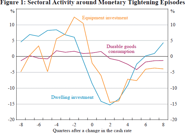
The main aim of this paper is to examine the extent to which interest sensitivity varies across different components of expenditure and production in Australia. Interestingly, Figure 1 suggests that among the expenditure components of GDP, dwelling investment and machinery & equipment investment tend to experience the most significant declines in activity following sustained increases in interest rates, while the fall in durable goods consumption is more moderate. This is in contrast to the US where, as mentioned earlier, machinery & equipment investment has been found to be less interest sensitive than residential investment and durable goods consumption.
The rest of the paper proceeds as follows. In Section 2 we outline the structural vector autoregression (SVAR) model of the Australian economy we use to analyse the sectoral effects of monetary policy. Section 3 then examines the effect of monetary policy shocks on the expenditure and production components of GDP. Section 4 analyses the effect of two other shocks to the system – a consumption shock and a foreign monetary policy shock – and assesses which shocks are most important in explaining the paths of the endogenous variables. In Section 5 we check the robustness of our results to different sample periods, potential-omitted variables and alternative identification assumptions. Section 6 offers some conclusions.