RDP 1999-04: Value at Risk: On the Stability and Forecasting of the Variance-Covariance Matrix 4. Forecast Performance
May 1999
- Download the Paper 604KB
There is a wide literature on modelling financial return variability. To date there has been little agreement in the findings of this literature. West and Cho (1994) compared the out-of-sample forecasting performance of univariate homoskedastic, GARCH, autoregressive and non-parametric models of exchange rate volatility to find that, over a one-week horizon, GARCH models tend to be slightly more accurate. However, for longer forecast horizons West and Cho found that there was little difference in the forecast performance of the various models. Similarly, Brailsford and Faff's (1996) analysis of Australian stock market variability provides some support for the use of GARCH modelling. However, the rankings of the various model forecasts are sensitive to the choice of performance criteria. In contrast Boudoukh, Richardson and Whitelaw (1997), in forecasting the volatility of US interest rates, found that a non-parametric approach outperformed the GARCH model. Campa and Chang (1997), also using foreign exchange data, found that, for shorter time horizons, exponentially weighted moving average models outperform both the fixed-weight historical and GARCH models. However, for longer forecast horizons, fixed-weight models are found to be superior.
More recently the literature has considered forecasts of covariances and correlations. Alexander and Leigh (1997), using equity and foreign exchange data, found that exponentially weighted moving average methods outperform fixed-weight and GARCH methods. It was noted in this study that GARCH models do not perform well when judged by statistical criteria that measure the centre of the distribution. Sheedy (1997) noted that, when comparing various GARCH-type models, the parsimonious models, such as the constant correlation model, perform as well as the more complicated specifications.
One-day-ahead forecasts and quarterly average forecasts are computed by moving the window lengths through the sample and re-estimating the models at each point (we consider moving windows of length 125 days, 250 days, 500 days, 750 days and 1,250 days). Due to the assumption of a zero mean, the one-day-ahead realised matrix will have the form:

and the elements of the quarterly (63 days) average realised matrix are calculated as:

Since past work has shown that model choice is sensitive to the performance criteria, when comparing the forecasts from the different models a number of performance measures are employed. If we assume conditional normality and zero mean, forecasting the variances and covariances is equivalent to forecasting the probability density function of returns. We can evaluate their accuracy by measuring how well the forecast distribution fits the actual data over the forecast horizon. The greater the log-likelihood function for a given sample the better is the fit of the estimated distribution.
In all cases, the exponentially weighted average log-likelihood falls significantly below the others. This is not unexpected since the parameter in this model is imposed and not estimated. When a window length of 250 days is used, the fixed-weight model outperforms the GARCH models, but when a window length of 1,250 days is used these rankings are reversed. Due to the large number of parameters that the GARCH models need to estimate, the length of data needed to obtain accurate parameter estimates is large. This is illustrated by the increased performance of the GARCH models when 1,250 days of data are used. The BEKK model outperforms the constant correlation based on its log-likelihood. This follows from the increased freedom of the parameterisation of the BEKK model.
Model comparisons based on the log-likelihood are conditional on the assumption of normality. As normality does not hold for many financial-return series, seven distribution-free performance measures are analysed.
Four symmetric performance criteria are considered:
| Mean error | 
|
| Mean absolute error | 
|
| Root mean squared error | 
|
| Mean absolute percentage error | 
|
The mean error offsets the effect of errors of different signs, however, the mean error can be used as a general guide as to the direction of over- or under-prediction. Both the mean absolute error and the root mean squared error (RMSE) focus on the magnitude of errors without taking into account the direction of error, with the RMSE placing greater weight on larger errors. The mean absolute percentage error gives a relative indication of overall forecasting performance.
To account for asymmetry in the loss function we use two error statistics developed by Brailsford and Faff (1996):
| Mean mixed error (under) | 
|
where o refers to number of over predictions and u to the number of under predictions
| Mean mixed error (over) | 
|
The mean mixed error (under) penalises under-predictions more heavily while the mean mixed error
(over) places greater weight on over-predictions. Finally, to test the efficiency of each model's
forecasts we consider the regression R2 from  .
If the model were fully efficient ϕ would not be significantly different from
zero, and δ and the R2 would both be close to one.
.
If the model were fully efficient ϕ would not be significantly different from
zero, and δ and the R2 would both be close to one.
At each point in time the rolling-window estimation results in a forecast variance-covariance matrix to be compared with the actual realisation. Given that the foreign exchange matrix contains 45 elements and the interest rate matrix contains 36 elements, rather than assess each model's forecast performance for each individual variance and covariance a more parsimonious approach was adopted. At each point in time each element of the variance-covariance matrix is treated as a separate observation. The forecast performance measures were then averaged across all observations. The results for the daily forecasts are summarised in Figures 2 and 3. For all criteria, the smaller the number the better (except the R-squared measure). Full details are reported in Appendix C.
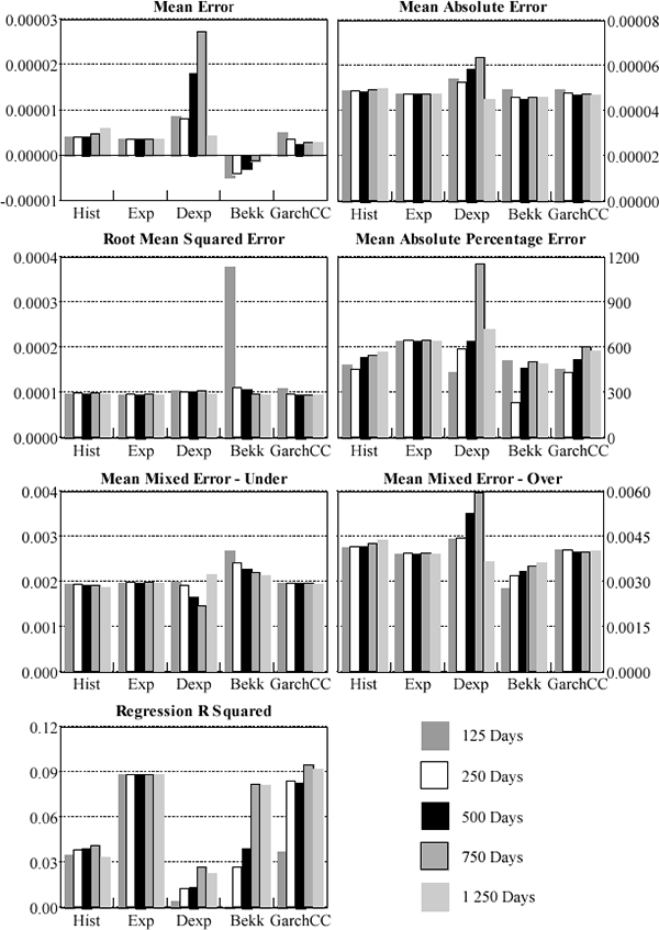
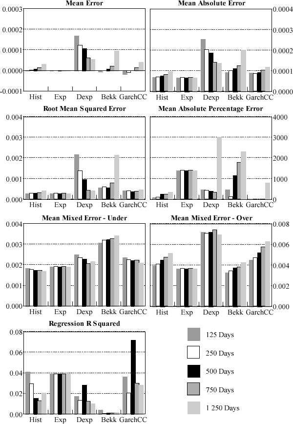
Clearly, model choice depends crucially on the metric used. Across criteria, no one model consistently outperforms any other. Given this variation, previous work that relies on one metric should be viewed with caution. In terms of mean error, mean absolute error, root mean squared error, mean under-prediction, and R-squared the simpler models (the fixed-weight and the static exponential models) are preferred. However, the GARCH models tend to do better when the models are assessed against the mean-absolute percentage error. Also the BEKK formulation of the GARCH model tends to produce the lowest average over-prediction (particularly for the foreign exchange data).
When the different models are compared across all metrics the more complicated GARCH models do not, in general, out-perform the simpler fixed-weight and exponentially weighted moving average approaches. For interest rates, the static exponentially weighted moving average model usually dominates all other models. For all criteria except the MAPE and MMEU the exponentially-weighted model performs best, both when forecasting daily and quarter-average variances and covariances. The fact that the fixed-parameter exponential model, in general, outperforms the dynamic exponential model provides quite strong evidence for the use of the constant parameter simplifying assumption used by RiskMetrics. The sharp decay in the weights of the static exponential model is such that the effective data window is quite short – lengthening the data window has little impact on the forecasted variances and covariances (this can be seen in Figure 3: the performance of the static model is invariant to the window length). This indicates that, for the interest rates' variance-covariance, shorter window lengths provide more efficient forecasts. This finding is consistent with the results of the diagnostic testing of the constant correlation model, which suggest that correlations tend to evolve gradually over time.
The relative performance of GARCH models is strongest in the case of the daily foreign-exchange forecasts. However, the differences in performance across models are not large and for shorter window lengths the simpler models tend to be favoured. The constant-parameter exponential moving average forecasts one-day-ahead variances and covariances performs well while the equally-weighted historical average performs relatively strongly in forecasting quarter-average variances and covariances. Although the simpler models' advantage dissipates as the window length is increased, the more complicated models do not then dominate. In conclusion, the simpler models apparently do not consistently under-perform their more complicated counterparts – in fact, there is some support for the contrary.
To test whether performance levels differ significantly across the five models we use the test of equality of the mean squared error values presented by West and Cho (1994). Under the null hypothesis of equality of mean squared errors, the test statistic has a χ2(4) distribution. The tests of equality are carried out on the daily and quarter-average forecasts for each of the different window lengths. Table 3 contains these results.
| Window length | 125 | 250 | 500 | 750 | 1,250 |
|---|---|---|---|---|---|
| Foreign exchange | |||||
| Daily forecast | 257.6* | 193.3* | 687.5* | 1,075.4* | 50.5* |
| Quarter average forecast | 461.7* | 959.0* | 2,009.2* | 4,220.3* | 1,028.0* |
| Interest rates | |||||
| Daily forecast | 11,797.8* | 3,304.9* | 81.6* | 186.2* | 201.7* |
| Quarter average forecast | 728.5* | 305.1* | 130.1* | 526.8* | 383.7* |
Note: * denotes significance at the 1 per cent level |
|||||
The null of equality is rejected in all cases. To further investigate the differences amongst models we applied West and Cho's test to other groupings of models. In most instances we found that each model produced a mean squared error that differed significantly from that of all other models. When considering daily foreign exchange variances and covariances based on a 125 day window, and daily interest rate forecasts using 125, 250 and 1,250 day calibration windows all models produced significantly different mean squared errors. Similarly, in the case of the quarter-average forecasts only one instance of equality was identified (the dynamic exponential, BEKK and constant-correlation models when applied to interest rates and calibrated on a 500 day window).
For the daily foreign exchange forecasts the model groupings based on mean squared errors vary across the different window lengths. When 250 or 500 day window lengths are used the West and Cho test groups together the dynamic exponential and BEKK models, and the fixed-weight, fixed-parameter exponential and constant-correlation models. Mean squared errors produced by the dynamic exponential, BEKK and fixed-weight models, and the fixed-parameter exponential and constant correlation models do not differ significantly when the 750 day window is used. For the 1,250 day window the fixed-weight and dynamic exponential models, and the fixed-parameter exponential, BEKK and constant-correlation models may be grouped together. In the case of the daily interest rate forecasts (500 and 750 day windows) the dynamic exponential and BEKK models, and the three other models may be grouped together.
In addition to testing across models we used the West and Cho test to test whether, for a given model, the mean squared errors differed significantly across the various data window lengths. The results of this testing are presented in Table 4.
| Model | Hist | Exp | Dexp | Bekk | GarchCC |
|---|---|---|---|---|---|
| Foreign exchange | |||||
| Daily forecast | 4.3 | 4.0 | 421.2* | 11.8** | 6.4 |
| Quarter average forecast | 1,189.9* | 4.0 | 833.2* | 5.1 | 7.0 |
| Interest rates | |||||
| Daily forecast | 115.2* | 4.0 | 60.8* | 9.3 | 292.3* |
| Quarter average forecast | 217.5* | 4.0 | 89.9* | 20.9* | 22.4* |
Notes: * and ** denotes significance at the 1 per cent and 5 per cent level respectively |
|||||
The effect of increasing the data window length varies across the different models. For the historical approach, the shorter the length of data used, the better the model (at least down to our smallest window of 125 days). For the quarter-average foreign exchange, daily interest rate and quarter-average interest rate forecasts the differences in mean squared errors are significant. The fixed-parameter exponentially-weighted moving average approach gains no benefit from increasing the data window, since little weight falls on data more than a quarter ago. The GARCH models do not consistently favour longer window lengths. For instance, in the case of the BEKK model, increasing the window length significantly reduces mean squared errors for daily foreign exchange forecasts, but significantly increases mean squared errors for quarter-average interest rate forecasts.
The fact that the forecast performance of the dynamic exponentially moving average and the GARCH models do not systematically improve as the length of data used for model estimation increases is a little surprising. Increased data length should provide more accurate parameter estimates. The fact that more precise parameter estimates are not resulting in more precise forecasts suggests that these may not be appropriate models for this purpose and that other classes of models should be considered.
Further analysis of forecast errors for the individual variances and covariances shows that much of the relatively poor forecasting performance of the GARCH models can be attributed to extremely poor prediction of a small number of elements within the variance-covariance matrix (for example, the variance of the Australian dollar – New Zealand dollar exchange rate). When these elements are removed, however, the GARCH models still do not outperform the simpler models. The simpler models exhibit fairly constant behaviour across the elements of the variance-covariance matrix. This is consistent across all forecast-error metrics. As the sample size is increased these simple models perform better on average across all matrix elements, but the dispersion around this average increases. This behaviour is found in both the daily and quarter-average results. For the GARCH models there does not seem to be a consistent relationship between the length of data window and the dispersion of forecasting accuracy across the elements of the variance-covariance matrix. At times increasing the data window increases the spread of forecast metrics across the matrix elements, while at other times the spread is reduced.
The users of a VaR model are not likely to view over- and under-prediction of variances and covariances equally. A model that consistently over-predicts volatility will overstate a portfolio's risk. This may be attractive to supervisors who may prefer models to err on the conservative side. However, individual traders within a firm may prefer models which under-predict risk and thus overstate risk-adjusted returns. It is not clear whether the banking firm as a whole would prefer a model that over- or under-predicts risk. The capital allocation flowing from an overly conservative model will be more expensive and hurdle rates of return unnecessarily high. Against this, a model that consistently under-predicts will expose the bank to an unexpectedly high probability of bankruptcy. We need to consider prediction of variances and correlations separately. Over-estimation of variances unambiguously over-predicts true risk. The effect of over-prediction of correlation depends upon the composition of the portfolio subject to the VaR model. Hence, we separately consider three measures of forecast bias in variance prediction: the mean error, and the mean mixed errors, both over and under. These are shown in Figures 4 and 5. Full details are given in Appendix C.
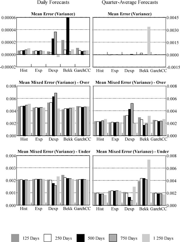
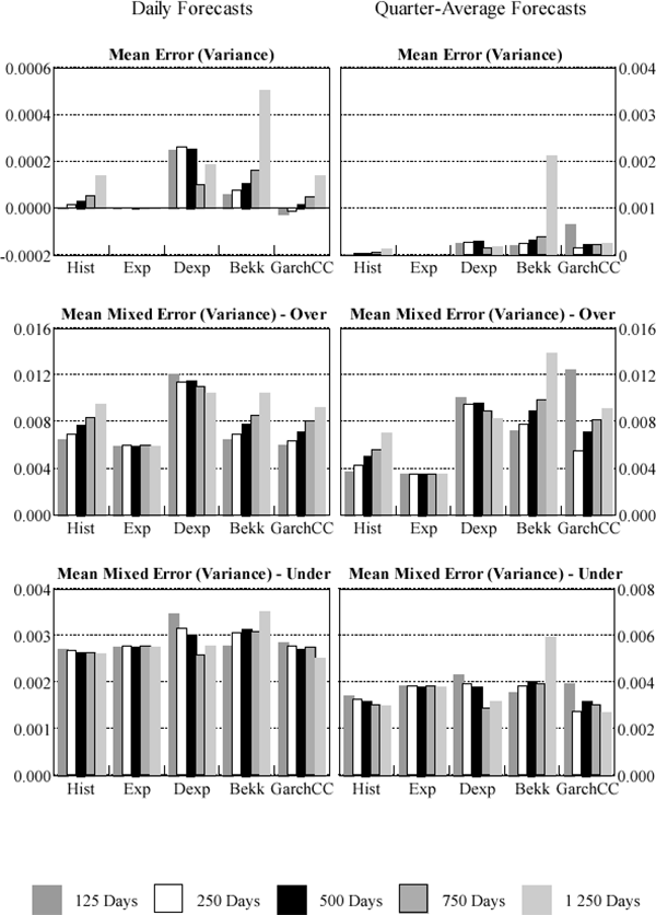
Consistent with the previous results, the fixed-parameter exponentially-weighted moving average tends to outperform the other models when forecasting interest rates, producing low mean-error and low over-prediction results. For daily and quarterly interest-rate variance forecasts the historical and constant-correlation GARCH models respectively provide the least under-prediction and thus can be taken to be the most conservative models. The results are more mixed for foreign exchange with no model consistently outperforming the others.
As we noted earlier, the frequency with which banks re-estimate their variance-covariance matrix varies. While banks are required to re-estimate the matrix at least quarterly for regulatory purposes, many banks update their matrix each day. To gauge the impact of less frequent re-estimation on forecast performance we compare the root mean squared error of one-day-ahead forecasts with that of the forecast for the last day of the quarter. The percentage increase in root mean squared error is shown in Table 5.
| Foreign exchange | Interest rates | |
|---|---|---|
| Fixed-weight historical | ||
| 125 | 2.21 | 2.12 |
| 250 | −1.42 | −1.14 |
| 500 | 0.44 | 0.25 |
| 750 | −2.67 | −2.92 |
| 1,250 | 2.32 | 2.18 |
| Exponential smoothing – fixed-parameter | ||
| 125 | 8.03 | 8.00 |
| 250 | 4.76 | 5.05 |
| 500 | 5.21 | 5.15 |
| 750 | 1.17 | 1.07 |
| 1,250 | 6.23 | 6.27 |
| Dynamic exponential smoothing | ||
| 125 | 11.19 | 11.32 |
| 250 | 7.39 | 7.84 |
| 500 | 6.12 | 6.17 |
| 750 | 2.46 | 2.44 |
| 1,250 | 6.73 | 6.80 |
| Constant correlation GARCH | ||
| 125 | 2,712.01 | 3,360.55 |
| 250 | 21.58 | 29.51 |
| 500 | −4.74 | −4.65 |
| 750 | 25.39 | 25.08 |
| 1,250 | 39.38 | 39.38 |
| BEKK GARCH | ||
| 125 | 33.21 | 38.53 |
| 250 | 238.23 | 293.77 |
| 500 | −1.53 | −1.39 |
| 750 | 50.69 | 50.41 |
| 1,250 | 50.50 | 51.52 |
Note: For each model and each element of the variance-covariance matrix the root mean squared error was calculated for forecasts of the variance or covariance to be observed on the next day and the last day of the quarter. This table shows the difference between the two root mean squared errors expressed as a percentage of the one-day-ahead root mean squared error. This ratio has been averaged across all elements of the variance-covariance matrix. |
||
The first three models predict that future variances and covariances will remain constant. The forecast accuracy of these simple models declines by something in the range of 2 to 10 per cent, which in comparison with the other measurement errors embodied in VaR models is probably not large (see, for example, Gizycki and Hereford (1998)). In contrast, the GARCH models (in which the future path of variances and covariances follows a smooth decay function) perform much more poorly over the longer forecast horizon. The poor performance of the models calibrated on the shorter data periods may be attributed to imprecision in estimation of the model parameters. However, the forecast accuracy of the more robust long-window estimates declines by as much as a half over the quarter. In several instances we obtain the unusual result that better forecast accuracy is obtained for the longer horizon than the day-ahead forecasts.