RDP 9812: An Optimising Model for Monetary Policy Analysis: Can Habit Formation Help? 4. Empirical Results
September 1998
- Download the Paper 395KB
Using the data detailed in Table 1, and estimating over the sample 1966:Q1 to 1995:Q4, I obtain the parameter estimates shown in the first column of Table 2. At the estimated parameter values, we find that: (1) habit formation is an economically important determinant in the utility function; (2) the habit formation reference level is essentially last period's consumption level; (3) rule-of-thumb behaviour is important, with about one-fourth of income accruing to rule-of-thumb consumers; (4) the intertemporal elasticity of substitution is quite small; (5) for those who look forward, the horizon is long; the parameter ρ takes the estimated value 0.996 on a quarterly basis, 0.984 on an annual basis; and (6) the model explains most, but not all, of the autocorrelation in the consumption data, as evidenced by the low p-value for the Ljung-Box test for serial correlation in the first 12 residual autocorrelations in the consumption equation.
| Baseline model | ||
|---|---|---|
| Coefficient | Estimate | Standard error |
| γ | 0.80 | 0.19 |
| ρz | 0.0015 | 0.0039 |
| λ | 0.26 | 0.13 |
| σ | 6.11 | 1.81 |
| ρ | 0.99 | 0.01 |
| δ | 28.49 | 5.17 |
| Ljung-Box Q(12) (p-value) | ||
| Consumption | 83.7 (0.00) | |
| Income | 6.1 (0.91) | |
| Federal funds rate | 13.5 (0.33) | |
| Inflation | 8.2 (0.77) | |
| Log-likelihood | 2,366.43 | |
| Detail on error correlations for consumption
equation (standard errors in parentheses) |
||
| Lag | Autocorrelation | Partial correlation |
| 1 | 0.55(0.14) | 0.55(0.09) |
| 2 | 0.39(0.14) | 0.12(0.09) |
| 3 | 0.42(0.14) | 0.25(0.09) |
| 4 | 0.15(0.14) | −0.27(0.09) |
The structural consumption equation error shows one significant autocorrelation of about 0.55. This correlation might be the manifestation of time-averaging in the data (Ermini 1989), or might reflect the durability of some components of consumption that are nonetheless classified as nondurables and services (Mankiw 1982). The standard errors reported in Table 1 are corrected for the estimated correlation in this error. However, all of the autocorrelation function computations, likelihood ratio tests, and simulations reported below assume the errors to be white. That is, none of the dynamics in the results reported below may be attributed to across-time correlation in the error terms.
The low estimated value of the parameter that indexes the ‘memory’ in the habit reference level, ρz, suggests that the operative reference level is last quarter's consumption. One presumes that habits are formed over horizons longer than one quarter, so this estimate of ρz is perhaps lower than expected.
However, the estimate can be justified on several grounds. First, if the level of (detrended) consumption exhibits significant autocorrelation, then last period's consumption contains information about consumption in previous periods. So the lagged level of consumption may have considerable ‘memory’ itself.
Second, note that rewriting the period utility function as:
and setting ρz = 0 yields the special case:
which shows that the essence of habit formation is that it mixes utility from the level of consumption with utility from the change in consumption. That is, the habit formation model with any normally shaped utility function will imply smoothing of both the level of consumption and its changes (provided γ is not zero). Larger values of ρz simply define the changes relative to a longer distributed lag of past consumption.[5]
Seen in this light, it becomes clear that a single lag of consumption in the reference level is sufficient to impart the smoothness to changes in consumption expenditures that is absent in the standard life-cycle model. In addition, note that the linearised consumption function with ρz = 0 is:
Note that the third term on the right-hand side, the weighted sum of expected future changes in consumption, will differ relatively little from the weighted sum of expected future deviations of consumption from a moving average of past consumption (the corresponding term in the consumption function with ρz ≠ 0). The difference will manifest itself for the most part in a small difference in the weights on future consumption changes. In essence, this specification of the habit formation model builds enough linkage between current consumption and future changes in consumption with or without a long memory in the reference level.[6]
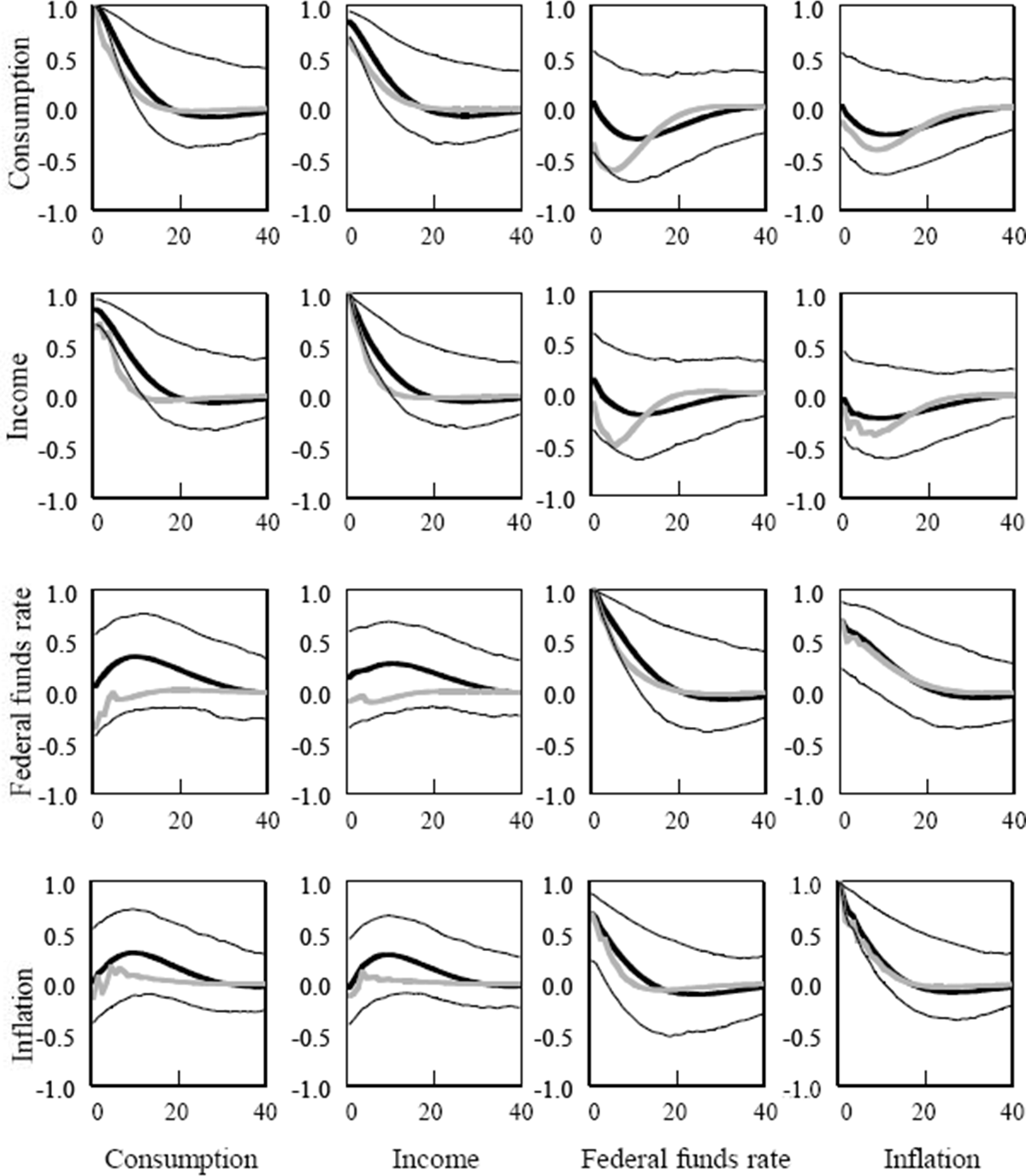
As I argue above, obtaining sensible parameter estimates is a necessary but not a sufficient condition for obtaining a reliable model for monetary policy analysis. Figure 1 displays the full set of autocovariances for the unconstrained VAR (the thick black lines) and the constrained consumption function (the grey lines). As the figure shows, the model has recovered the dynamic covariances for consumption expenditures quite well, capturing the persistence in the autocorrelation, as well as the persistent dynamic correlations between consumption and income, interest rates, and inflation.

Notes: Ordinate: lags in quarters. Co-ordinate: correlation function. Thick black lines, VAR; grey lines, constrained habit-formation model; thin black lines, VAR standard error bands.
The thin black lines in Figure 1 display the 90 per cent confidence intervals around the VAR's vector autocovariance function. As the plot shows, the differences between the two autocorrelation functions are generally insignificant at the 10 per cent level. Thus the correlations that the structural model cannot match are generally not precisely determined in the data. In Section 4.1 below, I perform a series of likelihood ratio tests to determine the statistical significance of a variety of restrictions on the model.[7]
4.1 Nested Tests of Habit Formation and Rule-of-thumb Behaviour
The hypothesis that habit formation is unimportant in this model – that the exponent γ on the reference level of consumption is zero – is overwhelmingly rejected. The χ2 likelihood ratio test for this single restriction takes the value 21.4, with p-value of 4×10⁻⁶. Similarly, the hypothesis that rule-of-thumb behaviour is unimportant is strongly rejected. The χ2 likelihood ratio test for the restriction λ = 0 takes the value 12.6, with p-value = 4×10⁻⁴. It is interesting to note that the likelihood ratio test for the constrained baseline model, which incorporates the many zero restrictions and cross-equation restrictions implied by the structure of the consumption model and by rational expectations, takes the value 32.8, not significant at even the 10 per cent level. This is one of relatively few cases in which the joint restrictions imposed by an optimisation-based model with rational expectations cannot be rejected relative to the unconstrained model in which the constrained model is nested.
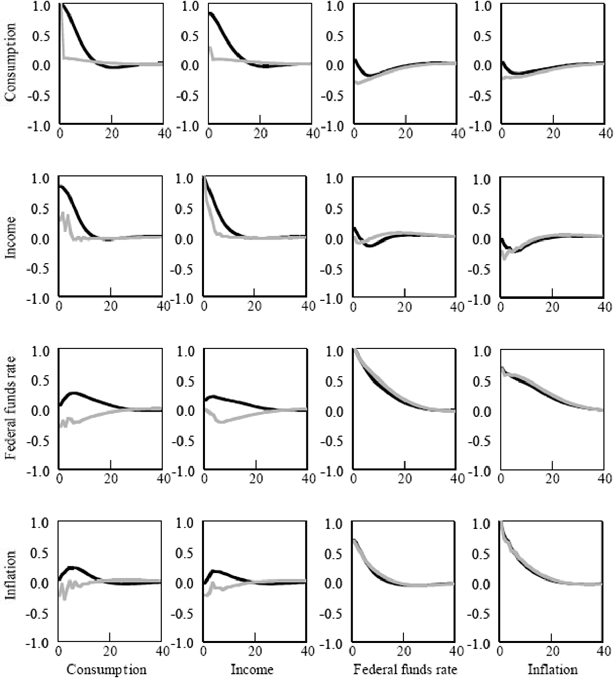
The vector autocovariance function illustrates the importance of habit formation and rule-of-thumb behaviour in replicating the dynamic interactions among consumption, income, interest rates and inflation. As Figure 2 shows, the primary consumption dynamics in the model that sets γ and λ to zero are almost totally missing. The simple PIH model cannot replicate the dynamics in the data. Both rule-of-thumb behaviour and habit formation are statistically significant modifications to add to the model.

Notes: Ordinate: lags in quarters. Co-ordinate: correlation function. Black lines, VAR; grey lines, constrained model.
4.2 Adding Restrictions to the Model
We now progressively add restrictions to the unconstrained portions of the model, in order to identify the systematic component of monetary policy and the pricing decisions of firms. I begin with the monetary policy function, imposing zero restrictions to the reduced-form funds rate equation so that it takes the form of a simple Taylor rule (1993):
where  and
and
 are the
equilibrium real interest rate and the inflation target, respectively. These simple restrictions
do not significantly deteriorate the likelihood from its baseline model value, and the vector
autocovariance function shows little sign that the imposition of the Taylor rule on the model
has constrained the dynamics in an economically significant way.
The second step is to constrain the price process. I begin by using a very simple version of a Fuhrer–Moore contracting model, which can be shown to be equivalent to a two-sided inflation specification (see Fuhrer and Moore (1992, 1995a) and Roberts (1997)):
This additional set of restrictions does not significantly deteriorate the likelihood from the baseline model's likelihood value. In addition, further constraining the price dynamics exactly as in Fuhrer and Moore (1995a), with explicit nominal price contracts, does not cause a statistically significant deterioration in the likelihood.
Finally, we allow the non-consumption components of GDP to enter the model. The importance of this addition is that the funds rate in the policy reaction function can now respond to the total GDP gap, rather than just consumption of nondurable goods and services. In addition, the overall GDP gap can drive the contract price specification. Other GDP is entered as in the earlier ‘I–S’ specification of Fuhrer and Moore (1995b). That is, the gap between non-consumption GDP and its trend depends positively on its own lag and negatively on the difference between the ex ante long-term (model-consistent) real rate and its equilibrium:
The addition of this equation and of the feedback of total GDP into interest rate and price determination does not significantly deteriorate the likelihood.
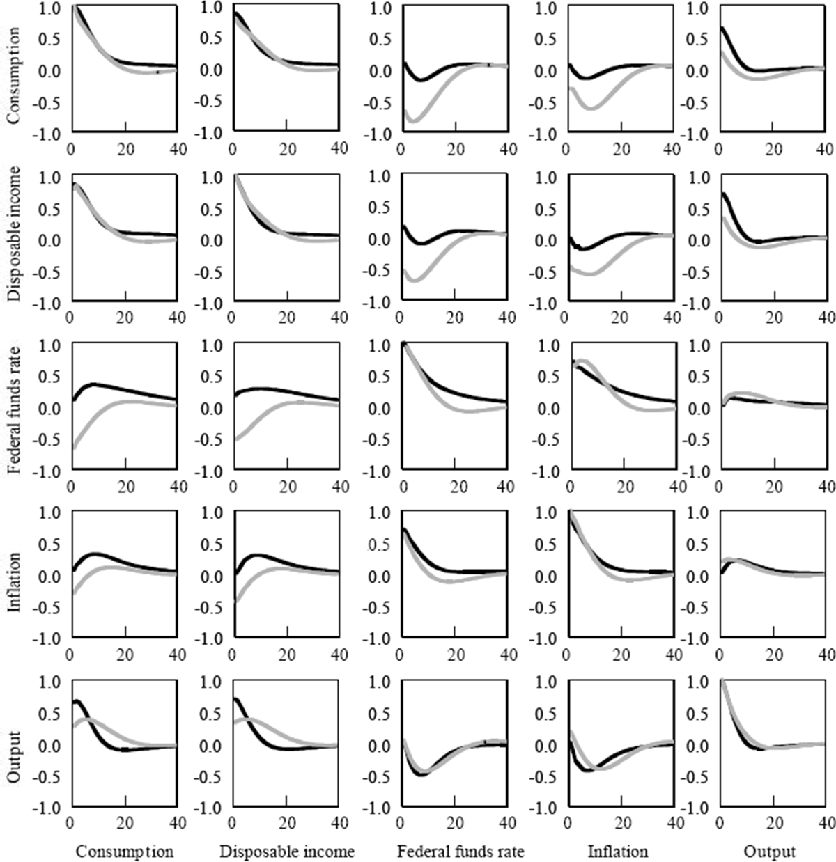
Figure 3 compares the vector autocovariance function for this more fully constrained (and identified) model with the unconstrained VAR autocovariance function. As the figure indicates, the constrained model largely replicates the dynamic behaviour of the unconstrained VAR. However, the model cannot perfectly replicate unconstrained dynamic behaviour. For example, while the correlation between consumption and the lagged funds rate or lagged inflation is negative, it is too strongly so. In addition, the correlation between the funds rate and lagged consumption is negative, while the VAR says it should be mildly positive. Recall, however, that these dynamic correlations are not so precisely determined in the VAR that the differences between the constrained model and the VAR are significant. In a sense, these autocorrelation comparisons provide graphical verification of the likelihood ratio tests conducted above.

Notes: Ordinate: lags in quarters. Co-ordinate: correlation function. Black lines, VAR; grey lines, habit-formation.
Footnotes
In this sense, the habit formation may provide a reasonable approximation to a model with a standard utility function and costs of adjustment in ΔCt [5]
The simulation presented in Figure 6 shows the effect of a longer-memory reference level on a standard disinflation simulation. [6]
The confidence intervals are computed as follows. I assume the distribution of coefficient estimates to be asymptotically normal. I follow a Monte Carlo technique that draws a vector of coefficient estimates from the multivariate normal distribution centred on the sample estimates, with covariance matrix as estimated from the sample. For each vector of estimates, I compute the corresponding vector autocovariance function, holding the residual covariance matrix fixed. The 90 per cent confidence intervals are bounded by the 5th and 95th percentiles of the ranked autocovariance functions. [7]


