RDP 9403: Capital Constraints and Employment 2. Techniques and Data
June 1994
- Download the Paper 109KB
This section describes the methods used to estimate full-capacity employment and the investment projections; it also describes the data used. Full-capacity employment is the labour that could be employed if the current capital stock was operated at full capacity. A two stage procedure is used to generate these estimates. The first stage estimates the capital-constrained output level. The second stage estimates the employment associated with this capacity constrained level of output, i.e. full-capacity employment. The projections of investment required for differing levels of employment growth are then made based upon assumptions about future capital to labour ratios.
2.1 Capacity Output
Methods of calculating capacity output are commonly ad hoc; for example, connecting peak levels of output together with a linear trend. The estimates of capacity output in this paper are based upon a method described in Berg (1984). Berg's method improves on others by explicitly basing capacity estimates on a ‘putty-clay’ production technology. With putty-clay technology the productive technique is freely chosen before installation but fixed after installation. Thus, although they can be altered before installation, the capital/labour/output ratios are fixed after installation.[4] This embodies the idea that once a machine is installed its output and the number of people required to use it cannot be altered. In this paper we allow for some post-installation, or ‘disembodied’, technical change. This possibility can capture physical depreciation as well as possible changes in the production technique. This description of technology is not specific to any particular production function but can be applied to any general function.
The exact production function used is not specified in this method. Instead, it is assumed that the capacity output to capital ratio follows a linear trend. This assumption can capture the effect of changing relative prices and technology upon the choice of capital intensity and, hence, capital productivity. This also requires an assumption that relative factor prices, or more specifically, future expectations of relative factor prices, change smoothly over the estimation period to be consistent with the trend in the capacity output to capital ratio. The capacity output, per hour, in year t, per unit of capital installed in year τ, is thus assumed to be:

where a0 is the capacity output per unit of capital installed in a base year t0, a1 is the change in this capacity output ratio between years and a2 captures any change in capacity output after installation.
The capacity output per hour in any given year is the sum of all active capital investments times the capacity output to capital ratios for those investments. The choice of what to include in the active capital stock will affect the estimates. There are many different assumptions that can be made about retirements of capital; we decided to keep the assumptions as simple as possible.[5] To this end we assume that all capital in a particular industry has a fixed life after which all investments are no longer productive, i.e. all retirements occur at the same age. The maximum life of capital used is based upon lives used by the ABS in its calculation of the capital stock. In most cases a life slightly shorter than that published in ABS Occasional Paper 1985/3 is used due to the gradual shortening of capital lives that has been occurring. The exact lives used for each sector are included in Table 1 which is presented in Section 3. We also assume that capital becomes productive the year after expenditure is incurred on it; this allows time for installation and integration into the output process. Thus the active capital stock includes all investments between the previous year and the maximum life of investment.
| Sector | Mean asset life for 60s | Life used (years) |
|---|---|---|
| Agriculture, forestry, fishing and hunting | 13 | 11 |
| Mining | 16 | 13 |
| Manufacturing | 19 | 16 |
| Electricity, gas and water | 22 | 18 |
| Construction | 13 | 11 |
| Wholesale and retail trade | 16 | 13 |
| Transport, storage and communication | 14 | 11 |
| Finance, property and business services | 13 | 9 |
| Recreation, personal and other services | 15 | 12 |
| Community services | 15 | 12 |
Multiplying the capacity output per hour by the maximum hours of operation of machines yields an estimate of capacity output. However, due to the lack of data on the maximum operation period of machines, we assume that the maximum operation period of machines is proportional to the normal hours of work in a given industry. We use average hours of work per person per week as an indicator of normal hours of work in an industry, scaling this up by a factor c to estimate the maximum operating period.
The capacity output in year t, Yt, can then be written as:
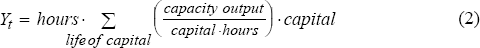
and in terms of more standard notation this can be written:
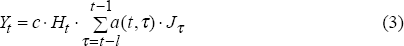
where c is the ratio between maximum operation period of the capital and normal hours of work, Ht are the normal hours of work in year t, l is the life of the capital and Jτ is gross investment in capital in year τ.
The estimation procedure involves choosing values for the ai coefficients in equation (1) to minimise an objective function subject to certain constraints. The objective used is to minimise the sum of differences between actual output and capacity output.[6] This fits the tightest capacity frontier to the data that is consistent with the underlying investment and hours data. The constraints used are that capacity output is always above actual output and that a(t,τ) is always positive, that is, investment cannot create negative output. This can be expressed as a linear programming problem:
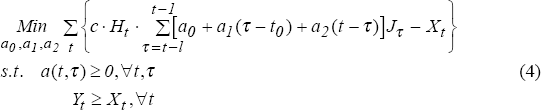
where Xt is actual output in year t. The estimation procedure is such that full output will occur in at least one year over the estimation period. This means that the estimates should be regarded as economic capacity rather than a strict engineering definition of capacity. They reflect the best efficiency that has been achieved over the estimation period. Thus, if the capital stock was never fully utilised during the estimation period, it is possible for greater capacity to exist than is estimated.
The assumption of putty-clay technology means that changes in relative prices have a limited effect on capacity output. As factor proportions are fixed after installation a change in relative factor prices should only affect the proportions embodied in current investment, not on the already installed capital stock. It is important to note though that changed relative factor prices would only lead to sub-optimal factor proportions if factor prices changed in an unexpected way. This is because future expectations should be included in previous investment decisions. The possibility of changes in relative factor prices affecting capacity output after installation is encompassed, in part, by the c·a2 parameter. However, this is subject to the assumption mentioned earlier, that relative factor prices change smoothly over the estimation period.
2.2 Full Capacity Employment
In estimating capacity employment there are two factors to be considered: actual employment can include some degree of surplus labour given current capital utilisation and some assumption needs to be made about the labour requirement on unused capital when it is fully utilised.
Two common methods have been used to estimate the quantity of surplus labour. One method is based on estimating production functions. The other assumes that labour productivity follows a well-defined trend; departures from this trend are then attributed to under-utilisation of labour.[7] The second approach is used here due to the difficulty encountered in fitting production functions across all sectors of the economy. We assume that productivity follows a quadratic time trend.[8] To estimate the productivity frontier a quadratic trend is fitted through each industry's productivity series and then shifted up by the amount of the largest positive difference.[9] The frontier generated indicates the best productivity that could have been achieved in the absence of any surplus labour. Using this measure the hours of work related to actual production can be calculated by dividing output by this frontier productivity measure. This can be converted to employment by making some assumption about what proportion of the surplus labour is full-time or part-time. For convenience we assume that surplus labour contains the same proportion of full-time and part-time labour as our estimated ‘productive’ employment.
The next step involves calculating the number of workers required to operate the installed capital at full capacity. The capacity output estimation procedure above allows us to estimate what proportion of the capital stock is in operation at any time. The estimation procedure generates capacity output to capital ratios for each vintage in each year. Assuming that recent investments are operated before older investments the capacity outputs from each vintage in a year, starting from the most recent, are added until they equal actual output for that year.[10] This identifies which vintages were probably used for production in that year. The total investment in these vintages is then summed and divided by the total stock to estimate a capital utilisation rate.[11] Full-capacity employment is then calculated by assuming that the capital to labour ratio on the idle units will be the same as on the units already in use in each particular year.[12]
The ‘productive’ employment calculated in the first stage is multiplied by the capital utilisation figure to estimate full-capacity employment. We emphasise that as this estimate does not include any surplus labour it is possible for this number to be less than actual employment, particularly in periods when surplus labour is estimated to be high. To the extent that this surplus labour is retained full capacity employment could be higher than the figure we indicate. Results from this method indicate that there is generally a higher labour requirement to increase output as older, less productive, machines are being used.
2.3 Investment Projections
The methods used allow us to determine the required rate of investment to sustain a given rate of employment growth. In projecting the required rate of investment a number of steps are followed.[13] First, we assume that the sectoral shares of employment continue to follow their current trends.[14] Next, projections of total employment in the future, based upon selected growth rates, are used to calculate employment in each sector based on the projected shares.
A capital to labour ratio is then calculated and we assume this also follows its trend. The capital stock is calculated by adding together the gross investment over the assumed life of capital in each sector. This is done as, even though depreciation is occurring, the labour required to operate a machine should not alter after installation. The machine may be less productive and break down more often but this affects the output to capital ratio not the capital to labour ratio. The labour supply used is the full employment value calculated earlier. The required capital stock is then calculated using the projections of the capital to labour ratio and employment.[15] The investment required to reach this stock level can then be calculated.
For the purposes of this paper three different growth rates of employment are considered. A baseline of 2.2 per cent growth per annum is used with high and low levels of 3.1 per cent and 1.4 per cent growth also considered. The high rate is chosen to correspond with the growth rate following the early 1980s recession and the other rates are arbitrarily chosen.
It is important to note that these projections are likely to be an overstatement of actual requirements for a number of reasons. An increase in the incidence of continuous operation of capital, concomitant with enterprise bargaining over working conditions, is likely to reduce the capital to output ratio and the capital to labour ratio. As this possibility is not included in the projections a lower level of capital would sustain a given level of employment. Also the recent recession may have reduced the relative cost of labour to capital, leading to a reduction in the desired capital intensity of production. This would also reduce the capital required to sustain a given level of employment; however, this effect would primarily apply to the newest investment due to the putty-clay production technology discussed above. In line with this the projections should be interpreted as an upper bound on investment requirements rather than as exact projections.
2.4 Data Sources
The techniques described above require data on output, investment, average hours worked and employment by industry. The estimation is applied to each of ten ASIC industry sectors and all estimations use data in 1989/90 constant prices.[16] Investment data across all of these sectors are only available on an annual basis so the data used are limited to this frequency.[17] Data on employment by industry are available from August 1966 so the estimation begins with the 1966/67 financial year.[18] The average hours data used are for employed persons; they are a weighted average of full-time and part-time workers. Investment data are available earlier than this and are used to construct a full stock of capital for the first estimation period.
The investment data used are gross fixed capital expenditure on plant and equipment for both public and private sectors from the Australian National Accounts. Plant and equipment data are used as this form of capital investment is most likely to include productive capital. Investment in non-dwelling construction would not generally be expected to directly raise the capacity output of a sector. While this form of investment may be necessary for output to be produced, a larger factory is unlikely to increase production in the same way that a larger metal press will.[19] Similarly, investment in roads and bridges may make it possible for output to be delivered to customers but will not increase the actual output potential (e.g. non-dwelling construction could be likened to the valve on a tap, opening it may increase the flow but not the actual supply). As physical depreciation can be encompassed in the estimation procedure, gross investment data are used rather than attempting to account for depreciation before estimation. Installation costs, which do not directly create productive capital, are included in the gross investment estimates. There is no reasonable way of accounting for these costs as estimates do not exist.[20] Nonetheless, if costs are proportional to the value of capital installed or small relative to the total investment, this should not affect the results.
Footnotes
The choice will be based on current and expected values of relative factor prices. [4]
The assumptions can be characterised by the shape of the retirement schedules, that is, a graph of capital retired against its age. The Australian Bureau of Statistics (ABS) assumes a bell shaped retirement function; thus most retirements occur close to a specific mean life while some capital lives for a relatively short or relatively long time. Other possible assumptions are that a fixed proportion of the investment is retired each year after some minimum age or that all retirements happen at the same age. [5]
It is also possible to consider other objectives such as minimising the sum of squared differences or log differences. These objectives will minimise the average divergence and proportional divergence respectively. A discussion of the effect of this is included with the results. [6]
This general approach was developed and popularised by Taylor (1976/1979). His basic method was to connect peaks in the productivity series to obtain the potential productivity series. These peak-to-peak methods suffer from endpoint problems and so a modified method in this general spirit is used. [7]
That is, a function of the form α + βt + γt2. Productivity is defined to be output divided by total hours worked. [8]
As this frontier touches at one point we need to assume that there is no surplus labour in at least one period in the estimation range. [9]
A fraction of the investment for the oldest year employed is used to ensure that the capacity output sum is exactly the same as actual output rather than slightly above or below it. [10]
This will not necessarily be the same as the capacity utilisation rate since the capacity output to capital ratio changes over time and the life of investment. [11]
This does not fix the capital to labour ratio between years; in fact the capital to labour ratio generally follows an upward trend over the estimation period. [12]
These projections are not forecasts of what we think will occur to investment in each year. They are projections, based on hypothetical scenarios, conditional on our assumptions and the structure of the model. [13]
For example, manufacturing's share of employment is falling while service sectors have rising shares. [14]
Actual employment was used to forecast shares of employment so, due to the slightly different numbers involved, employment growth in each sector is added onto the full employment bases rather than actual employment. [15]
The sectors examined are: Agriculture, Forestry, Fishing and Hunting; Mining; Manufacturing; Electricity, Gas and Water; Construction; Wholesale and Retail Trade; Transport, Storage and Communication; Finance, Property and Business Services; Community Services; Recreation, Personal and Other Services. The only major ASIC sector excluded is Public Administration and Defence as there are no investment data available for this sector. [16]
Quarterly investment data are available from Private New Capital Expenditure, Australia (ABS Cat. 5626.0), however, this only reports investment for a few industry subdivisions and is thus unsuitable for this project. [17]
The particular employment series used are total persons (full-time and part-time) from ABS Cat. No. 6203.0. [18]
Estimates were made using non-dwelling construction investment as well as plant and equipment investment. However, these estimates were not significantly different from the estimates using plant and equipment data only. Furthermore, non-dwelling construction investment generally follows the same pattern as plant and equipment investment or is relatively flat over time. As such it does not offer much additional information for fitting capacity output frontiers. [19]
The ABS publishes capital consumption; however, this is a measure of depreciation of the total capital stock rather than a measure of installation costs. [20]