Research Discussion Paper – RDP 2023-06 Firms' Price-setting Behaviour: Insights from Earnings Calls
1. Introduction
As observed in other advanced economies, consumer price inflation in Australia has been unusually high in recent years. While demand conditions have played an important role, supply-side factors have been the biggest driver of recent inflation outcomes and have been front of mind for company executives and policymakers (Figure 1).[1] The impact of upstream supply shocks on prices are generally not well captured by inflation models, so alternative and timely sources of information have become more important in assessing the inflation outlook. For this reason, policymakers have been closely monitoring firms' price-setting behaviour using insights derived from business liaisons and surveys of firms.
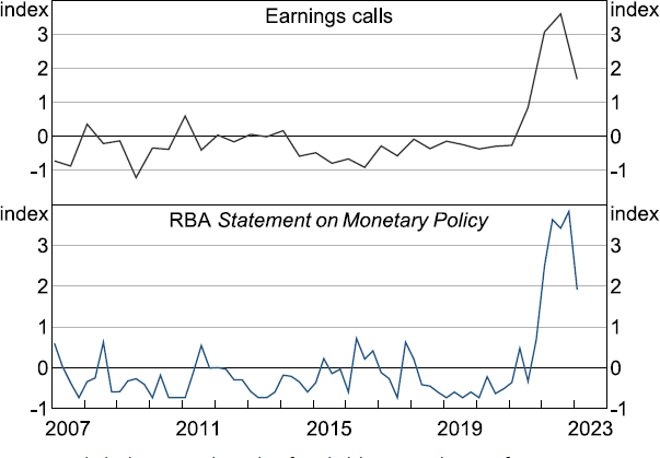
Note: Series are standardised to measure the number of standard deviations each series is from its average.
Sources: Authors' calculations; RBA; Reuters.
In this paper, we examine firms' price-setting behaviour by listening into what companies are saying about input costs, demand and final prices during their earnings calls. To do this, we use modern techniques in natural language processing (NLP) applied to listed Australian firms' earnings call transcripts. This approach allows us to systematically analyse firms' first-hand experiences with cost pressures and the effect this is having on their price-setting decisions.
Before the fact, it is unclear whether earnings calls, business liaison information or survey indicators reveal the most information about the pricing behaviour of firms. At the outset, our view is that each source has its own strengths and weaknesses, and it is the accretion of information from all three that is most useful to policymakers. Earnings calls provide consistent firm-level information over time, track a large number of firms and – using the new methodology outlined in this paper – allow analysts to construct a huge variety of different indices to monitor over time. However, the sample is restricted to larger listed companies and the information is only updated during earnings season. Business liaisons are timelier, but the composition of firms changes from period to period and responses are influenced by the types of questions being asked. Finally, existing business survey indicators provide consistent information over time, but sample sizes tend to be smaller, firm-level information is unavailable and policymakers are restricted to analysing a small number of pre-existing indicators.
To build our firm-level indices, we mine the text of listed Australian firms' earnings calls, starting from 2007. Sentiment indices are developed from the transcripts, covering various input costs, demand and final prices. This is done using two techniques. The first is a simple dictionary-based approach with each word coming from new dictionaries developed in consultation with policy experts from the Reserve Bank of Australia's Economic Analysis Department and supplemented using word embeddings. These dictionaries are available for download in the online Supplementary Information. The second, and preferred approach, draws on state-of-the-art machine learning models (zero-shot text classifiers) to uncover semantic meaning and identify when company executives are talking about our topics of interest. A subset of forward-looking indices is also developed. We experiment with two techniques to do this. First, we use recently developed algorithms to identify the tense being used in various sections of the earnings calls and then restrict our analysis to the parts of speech that are forward looking. Second, we use transformer-based machine learning classifiers to identify sections of the transcripts that are delivered in the future tense.
Using our newly constructed indices, this paper contributes to our analysis of current economic conditions in several ways. We show that the signal from these indices about input costs, demand and final prices is contemporaneous with the information the Reserve Bank of Australia receives as part of its extensive business liaison program and can help predict (in the sense of Granger causality) signals provided by regular firm-level surveys of business conditions. These results are consistent with a simple conceptual framework we use to explain why there is real-time information in earnings calls. Moreover, past information in our sentiment indices for input costs and final prices can help predict (again, in the sense of Granger causality) official statistics for producer and consumer price inflation in the reference period – that is, ignoring lags in the publication of these official statistics. Establishing that our new indicators track current economic conditions is helpful because, using the flexible methodology outlined in this paper, earnings calls can be used to construct a host of firm-level indicators that may not be available from other sources.
Using firm-level regressions we also document several facts about firms' price-setting behaviour that are relevant for policymakers in understanding the dynamics of the inflation process. We do not establish causal relationships but uncover interesting conditional correlations. In particular, we have four key findings related to the sensitivity, or elasticity, of sentiment about final prices to input costs and demand, after controlling for the effects of shocks that are common to all firms, including global supply shocks:
- First, final price sentiment has a stronger association with sentiment about input costs compared to sentiment about demand. This association is consistent with survey-based findings that the predominant pricing strategy of firms is to set prices as a mark-up over costs (Park, Rayner and D'Arcy 2010).
- Second, we find that firms react more to increasing input costs compared to decreasing input costs, suggesting that rising prices are likely to remain front of mind for company executives even as supply pressures moderate. This asymmetry is consistent with the type of firm-level behaviour reported in Peltzman (2000) and Pitschner (2020), who show that cost shocks matter much more for price increases.
- Third, we show that discussions around final prices have become more sensitive to sentiment regarding import costs in the post-COVID-19 environment but seem less sensitive to rising labour costs.
- Finally, we show the association between price-setting sentiment and input cost/demand sentiment differs significantly across industries, highlighting significant heterogeneity in firms' price-setting intentions.
Our paper also makes a methodological contribution to the literature. There is a growing body of research using earnings calls for macroeconomic analysis. For example, quarterly earnings calls have been used to analyse firm-level climate exposures (Sautner et al 2023), cyber risk exposures (Jamilov, Rey and Tahoun 2021), political risk exposures (Hassan et al 2019), sources of country risk (Hassan et al 2021) and the diffusion of disruptive technologies (Bloom et al 2021). All of these papers rely on matching documents to curated lists of keywords in order to identify topics of interest in the transcripts. Instead, ours is the first paper (to our knowledge) that uses a class of transformer-based machine learning models called zero-shot classifiers to classify earnings calls into our topics of interest. The classifier we use can be used to classify documents into any arbitrary set of themes. These classifiers are based on a powerful transformer-based neural machine translation architecture which has swept through the NLP landscape (O'Neill et al 2021; Ash and Hansen 2023), most prominently through the recent release of ChatGPT.
Finally, we make an economic contribution. The significant heterogeneity in pricing behaviour that we document has implications for macroeconomic models. Our findings suggest that the tone of firms' discussions about final prices depends on the source of the shocks firms face (demand or cost driven) as well as the direction of the shock, with firms' appearing to react more to cost increases relative to decreases. The latter finding suggests the assumption of symmetry in some price-setting models used in applied macroeconomics could be revisited. Our results also show that some industries seem much more responsive to changes in input costs and demand conditions relative to other industries. This underscores the importance of continuing to develop rich multisector models of the economy to better understand firms' reactions to different types of shocks, such as that developed by Rees (2020).
2. Data
Firms' earnings call transcripts are obtained from Reuters. The transcripts include both prepared remarks and subsequent question-and-answer (Q&A) sessions. Earnings calls typically take place a few hours after the release of earnings results. Earnings calls are a way for company executives to relay information to all interested parties, including the media, institutional and individual investors, and analysts from funds that manage money and sell financial products. In the calls, company executives deliver prepared remarks summarising the overall business position of the firm and the operating environment. This is then followed by a Q&A session where all interested parties ask questions about the outlook or probe into other issues. The information in these exchanges can be much richer than the prepared remarks alone.
Firms that hold earnings calls tend to be larger, with active investor bases that expect regular verbal updates and the opportunity to ask questions. There are around 550 distinct companies in our database and our analysis begins in 2007 (Figure 2). In total we work with around 5,500 transcripts, processing and analysing over 700,000 paragraphs along the way. Most firms release their results and hold earnings calls at a six-monthly frequency though some report quarterly or annually. Around 80 per cent of firms' reporting periods finish on 30 June and 31 December, with results released around two months later (Figure 3, top panel). A further 10 per cent of firms are so-called off-cycle reporters, whose reporting year ends in September, with the remainder reporting in other months throughout the year. The industry composition of the sample reflects the industrial composition of Australia's publicly listed companies (Figure 3, bottom panel). All our indices are constructed at the transcript level and then aggregated with no weighting scheme applied.
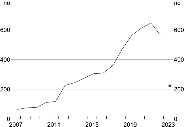
Note: Information for 2023 is up to end February only.
Source: Reuters.
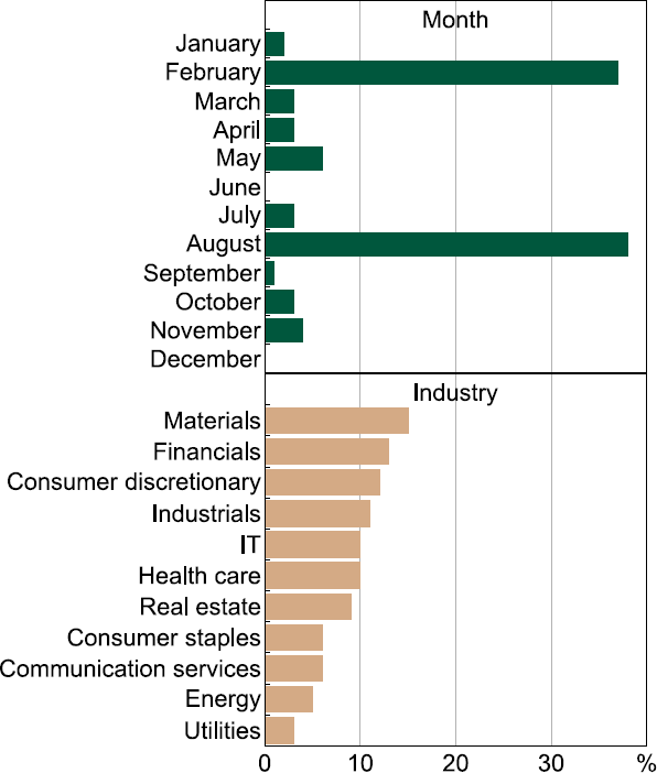
Source: Reuters.
3. Index Construction
We construct several sentiment indices from the text of each earnings call: (1) an input-cost sentiment index (including input cost subindices, such as that for labour costs); (2) a demand sentiment index; and (3) a final price sentiment index.[2]
To construct the indices, we use two approaches. The first is dictionary-based. We construct transcript-level sentiment indices by simply looking up specific dictionary terms in each of the earnings call transcripts. These dictionaries are put together in consultation with expert staff from the Reserve Bank of Australia's ‘Prices, Wages and Labour’ team. We also add additional ‘missing’ words to some of the dictionaries after training a word embedding model (Word2Vec). For example, the word ‘debottlenecking’ was originally missing from our general input cost dictionary but was added after embedding the word ‘bottleneck’ and using the embedding space to find semantically ‘nearby’ terms. After finalising the dictionary, we then conduct a proximity search anywhere within the sentence in which the dictionary term appears to look for qualifiers that indicate an increase or a decrease. After identifying the specific words in connection with their qualifiers, we sum the ‘hits’, take the balance of references to ‘increases’ and ‘decreases’, and divide it by the total number of words in the transcript. In total there are 70 terms related to input costs in the dictionary, which can be mapped into 10 input cost subindices (see Appendix A for details). We also develop separate dictionaries for consumer demand and final prices.
Specifically, letting Wit = [w1,w2,w3,...,wn] be a list of the words (with repetitions included as separate elements) used in firm i's transcript in time t, and Sit =[s1,s2,s3,...,sn] be the list of sentences, the dictionary-based sentiment index, DS, is calculated as:
where is the indicator function that is equal to one if the associated condition is met. Here, for a given sentence, s, and word, w, we record a positive contribution to the index if the word is a member of the relevant dictionary d, , and there is a qualifier in the selected sentence that indicates an increase, , without an offsetting negative qualifier that indicates a decrease,.
To illustrate the methodology, Table 1 includes random examples underlying the construction of the general input cost, labour cost, demand and final price indices.
| Company | Sentence | Relevant index | Keyword and qualifier |
|---|---|---|---|
| BlueScope Steel | Question: First of all, seeing a lot of publicity about the, not only the cost increase for EAF electrodes, but a great shortage and people struggling to get them. | General input costs | cost + increase |
| Commonwealth Bank | Prepared remark: However, because we're now doing better and because the economy is improved, we've passed on a 2% wage increase to our staff with effect from 1 January. | Labour costs | labour cost + increase |
| BHP Group | Prepared remark: In the past year we've continued to see demand for our products remain strong. | Demand | demand + strong |
| Tabcorp | Response: And with the price increase, all of the dividends through all of the divisions will increase commensurate with the price increase. | Final prices | price + increase |
|
Sources: Authors' calculations; Reuters |
|||
The benefit of the dictionary-based approach is that it is completely transparent. However, the process of developing dictionaries is manual and has several limitations. First, the dictionaries we develop are non-exhaustive, giving rise to many missed ‘hits’ or false negatives. Second, the simple dictionary-based approach does not capture semantic meaning, potentially giving rise to a significant number of false positives. Finally, as different companies use different specialised language it is difficult to develop a uniform dictionary, which could potentially generate inconsistent results. Ultimately, selecting an optimal set of keywords is a near impossible task and can bias inferences (King, Lam and Roberts 2017). For this reason, we use results from the dictionary-based approach in this paper as a crosscheck on those we obtain from a large language model.
Our second (and preferred) approach draws on a new generation of machine learning based large language models to uncover semantic meaning, which we use to identify when company executives are talking about our topics of interest. Our chosen topics of interest cover: hiring difficulties; supply shortages; labour costs increasing; labour costs decreasing; transportation costs increasing; transportation costs decreasing; import costs increasing; import costs decreasing; general input costs increasing; general input costs decreasing; final prices increasing; final prices decreasing; consumer demand increasing; and consumer demand decreasing. We parse the text of every paragraph in the transcripts (around 700,000 in total) and use the classifier to determine the probability the paragraph is about each of our topics of interest independently. The output from this process is illustrated in Figure 4, which demonstrates the model's ability to classify without finding explicit keyword matches. For example, the semantics of staff retention difficulties mentioned in the text from Australia's largest airline are captured by the model in classifying the theme hiring difficulties. In this way, we effectively reframe the dictionary-based approach into a text classification problem, enabling us to classify paragraphs without finding explicit keyword matches.
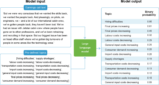
In this application, we apply a label to a paragraph if the model assigns the label a binary probability of greater than 70 per cent.[3] The sentiment index for a given topic is then calculated as the number of labelled paragraphs in a transcript divided by the total number of paragraphs. Specifically, letting p represent a paragraph from the list of all paragraphs Pit = [p1, p2, p3,...,pn] in firm i's transcript, the classification-based sentiment index, CS, for topic z, is calculated as:
where the indicator function is equal to one if there is a greater than 70 per cent probability the paragraph is about the topic of interest. The index nets off positive, , and negative, , references to a given topic.
To perform this classification, we use a class of deep learning models called zero-shot text classifiers. Zero-shot text classification refers to the ability of a model to classify text into an arbitrary set of user-chosen categories, even if it has not been explicitly trained on those categories. In other words, it can predict the correct label for a given input without any prior training data specific to that label. We use a complex 400-million-parameter zero-shot classifier developed by Facebook AI named BART-large-MNLI.[4] As the name suggests, there are two parts to the classifier.
‘BART-large’ refers to a large-scale pre-trained model called ‘BART’, short for Bidirectional and AutoRegressive Transformers. BART is based on a transformer architecture (Lewis et al 2019), which enables it to be trained at massive scale. In this case, the model develops an understanding of language semantics through training on English language free-text datasets, including the Wikipedia corpus, news and books.[5] The model's training objective is to minimise the loss associated with reconstructing corrupted sentences into their original form, learning the dependencies and context of natural language along the way.[6]
The second part of the classifier ‘MNLI’, stands for Multi-Genre Natural Language Inference. This refers to a clever training objective designed to fine-tune BART's ability to understand natural language. Following the procedure outlined in Yin, Hay and Roth (2019), BART is fine-tuned by tasking it with predicting the labels in the multi-nli dataset (see <https://huggingface.co/datasets/multi_nli>). This dataset is a crowd-sourced collection of sentence pairs from various genres, with each pair consisting of a premise and a hypothesis along with a label from one of the following categories: (1) ‘entailment’, whereby a human reading the premise would infer that the hypothesis is most likely to be true; (2) ‘contradiction’, whereby a human reading the premise would infer that the hypothesis is most likely to be false; and (3) ‘neutral’, indicating there is no discernible relationship of entailment or contradiction between the premise and the hypothesis. Fine-tuning BART to predict these class labels enables it to be used off-the-shelf as a zero-shot text classifier, as we do in this paper. We choose to use the BART-large-MNLI model specifically because it is fine-tuned for natural language inferencing.[7]
4. Index Validation
4.1 Expected information content
First and foremost, earnings calls are backward looking: they cover financial results for the previous six months and are delivered with a two-month lag. Taking this as our starting point, it is important to consider why the aggregate sentiment indices we develop would contain any information that is relevant for assessing current economic conditions. That is, it is important to ask why aggregate indices derived from earnings calls would contain any information that is already available in real-time indicators of current economic conditions taken from surveys of businesses or from business liaison programs, such as those run by central banks. If insights from earnings calls about current economic conditions are contemporaneous or help predict insights from survey respondents or liaison contacts from a similar set of businesses, then earnings calls must influence these respondents in some way. In this section, we argue there are three reasons this might occur.
- First, and most obvious, is that executives do, at times, reveal new facts about the current operating environment or the outlook. For example, executives of commercial banks often provide updates and forecasts for net interest margins over the year ahead. Forward-looking information is also elicited as part of the Q&A sessions.
- Second, executives often reveal new facts about decision-making processes, prompting a reassessment of the outlook. For instance, an executive could reveal that some divisional managers have been requested to reduce costs on an ongoing basis, thereby explaining persistent declines in expenses.
- Third, the clear and concise synthesis of existing information provided by executives during the earnings presentation and Q&A session could cause the outlook of others – such as business survey respondents or business liaison contacts – to be updated or revised through a process of fact-free learning (Aragones et al 2005).
The first two reasons require little explanation. New facts are presented, integrated into an existing knowledge base and the assessment of current and future economic conditions is modified. Within a Bayesian framework, these modifications are done mechanically according to Bayes' rule.
The third requires some explanation. We argue that executives can also change the assessment of current conditions as well as the outlook without communicating new facts, but by pointing out new regularities in an existing set of information and explaining how these are used to make decisions. For example, consider a survey respondent or business liaison contact seeking to understand why its firm increased prices by appealing to the macroeconomic determinants of the decision, which come from readily available information. The respondent favours a clear and concise explanation because they need to communicate this information to others. We argue the complexity of delivering a clear and concise explanation – that is, choosing a small number of explanatory factors out of a large set of possible candidates to achieve a given level of explainability – means that simple regularities based on existing facts are often overlooked (Aragones et al 2005). Once these regularities are clearly explained by their firm executives in the earnings calls, the logic can seem evident, and causes an update of the outlook due to a reassessment about how decisions will be made in the future.
This process of fact-free learning from earnings calls has parallels with recent explanations for why central bank communication can change the market's assessment of current economic conditions – the so-called ‘communication channel’ of monetary policy. Bauer and Swanson (2020) argue that a differential assessment of publicly available information between the central bank and the private sector can cause the private sector to revise its outlook, which the authors term the ‘response to news’ channel. For instance, the central bank could be putting a different weight on certain variables at different times to explain why particular decisions were made. Regardless of the precise mechanism, both explanations highlight why an expert evaluation of publicly available data can change an assessment of current economic conditions.
The three reasons outlined above give rise to some simple testable hypotheses, which if confirmed, would suggest there is contemporaneous or forward-looking information in the earnings call transcripts that is useful for understanding firms' price-setting behaviour:
- H1: the indices should have a strong contemporaneous or leading relationship with regular surveys of firms designed specifically to measure business conditions, including with respect to our concepts of interest (e.g. input costs, demand and final prices).
- H2: the indices should have a strong contemporaneous or leading relationship with similar real-time information obtained from the Reserve Bank of Australia's extensive business liaison program.
Confirming these hypotheses only provides suggestive evidence of the existence of real-time information in the earnings calls that is relevant for assessing current economic conditions. It could also be the case that earnings calls, regular surveys of firms and the information extracted from business liaisons are all similarly backward looking. To address this, we also examine whether our indices have a strong contemporaneous (or predictive) relationship with related official statistical measures in their reference quarter.[8]
4.2 Results
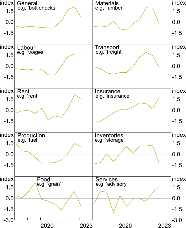
Before testing the hypotheses above, we first describe the usefulness of our aggregate indices as a narrative tool for explaining aggregate fluctuations in economic conditions. Figure 5 shows that the aggregate indices from both methodologies can identify significant turning points in the economy. For instance, all three indices (input costs, final prices and demand) fell sharply during the global financial crisis of 2008 and at the onset of the pandemic and have increased sharply since the middle of 2021. Sentiment regarding demand, prices and input costs has moderated lately, with the demand index identified using the zero-shot text classifier leading the declines in the price indices. This same dynamic also occurred following the global financial crisis. Disaggregated input cost indices from the zero-shot classifier are also consistent with recent developments, with sizable increases in references to general supply shortages, hiring difficulties and labour costs (Figure 6). In addition to this, the dictionary-based subindices show large increases in concerns related to rents (Figure A1).
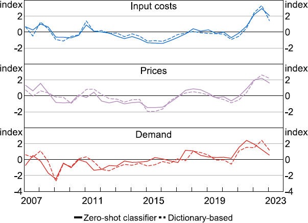
Note: Series are standardised to measure the number of standard deviations each series is from its mean value.
Sources: Authors' calculations; Reuters.
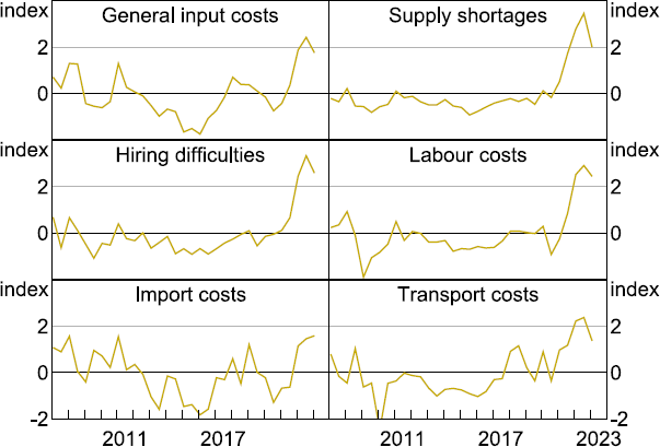
Note: Series are standardised to measure the number of standard deviations each series is from its mean value.
Sources: Authors' calculations; Reuters.
To perform a preliminary test of our hypotheses above about the timeliness of the information derived from earnings calls, Figure 7 compares sentiment indices obtained from the earnings calls to those constructed from two other sources.
- The Reserve Bank of Australia's business liaison program – this is a formal program of economic intelligence gathering established over 20 years ago, through which Reserve Bank of Australia staff meet frequently with firms from a pool of around 900 active contacts (Dwyer, McLoughlin and Walker 2022). Details of these discussions are systematically recorded in confidential ‘diary notes’. We use the text of these notes to construct indices for input costs, demand, final prices and labour costs using a similar approach as that applied to firms' earnings calls.
- A monthly survey of around 400 firms from the National Australia Bank (NAB) – this is a survey designed to produce statistical indices related to business conditions. We compare our text-based indices to the NAB survey-based indices for purchase costs, forward orders, selling prices and labour costs.
As shown in Figure 7, all three series – from earnings calls, business liaison and business surveys – appear tightly associated, hinting that there is real-time information in the earnings calls that is relevant for assessing current economic conditions.[9]
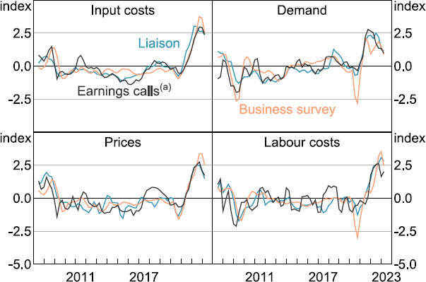
Notes:
Series are standardised to measure the number of standard deviations each series is from its mean value.
Rolling quarterly six-month average.
(a) Zero-shot classifier.
Sources: Authors' calculations; NAB; RBA; Reuters.
To test our hypotheses more formally, Table 2 shows the results of statistical tests for predictive or contemporaneous relationships. Our sentiment indices for input costs, demand, labour costs and prices are compared to comparable indices derived from business liaison and business surveys. In doing so, we do not account for publication lags in the release of the business survey indices (which are typically released with a three-week lag). In addition to this, the sentiment indices for input costs, demand, labour costs and final prices are compared to official statistics for growth in producer prices (PPI), domestic final demand (DFD), compensation of employees (COE) and consumer prices (CPI), respectively. Again, in these comparisons we pretend data on growth in the PPI, DFD, COE and the CPI are available immediately after the end of the quarter. That is, we assume there is no lag in the release of these statistics, while in reality there is a sizable publication lag.
The key finding from this exercise, before going into the details below, is that there is robust evidence information derived from earnings calls is contemporaneous with real-time updates received from the Reserve Bank of Australia's business contacts, regular business conditions surveys and with related statistical measures. This is consistent with the hypothesis that information from the earnings calls is relevant for assessing current economic conditions.
More specifically, Table 2 shows the results of bivariate Granger causality tests between the indices derived from earnings calls and their counterparts from either business conditions surveys, the Reserve Bank of Australia's business liaison or from related statistical releases.[10] To do this we run 12 bivariate VARs of the form:
where yt is the measure of interest. For example, in the first regression, yt includes the input cost sentiment index from earnings calls and the related measure from a survey of firms' purchase costs, with the results shown in the first row of Table 2. In the second regression, yt includes the input cost sentiment index from earnings calls and the related measure from the business liaison program, with the result shown in the second row of Table 2, and so on and so forth. The procedure we use to establish Granger causality follows Toda and Yamamoto (1995), using information criterion to determine the appropriate maximum lag length for the variables. Importantly, by including lagged values of both series, this approach deals with serial correlation in the macroeconomic situation, which might explain how backward-looking indicators may still have predictive power for future variables. The results in Table 2 restricts the analysis to the March and September quarters only, which is when most firms hold their earnings calls. Using quarter-end dates puts the earnings calls at a slight informational disadvantage, as the main reporting season occurs over the month of February and August, one month before the end of the quarter.
In the comparison with business surveys there is evidence that past information from the sentiment indices can help to predict future values. That is, the sentiment indices from earnings calls ‘Granger cause’ their conceptual counterparts from the business conditions survey (except for the series for selling prices). In the comparison with business liaison, the sentiment indices for input costs and demand are useful for predicting information from liaison; however, past information in liaison about labour costs and final prices appears informative for future information extracted from earnings calls. In the comparison against official statistical measures, the sentiment indices for input costs and final prices can help predict official statistics for growth in the PPI and CPI in the reference period. Finally, the last column of Table 2 shows peak correlations between each of the series and the period in which these occur. Peak correlations all occur in the same period, except for the input cost index, with the peak correlation occurring when liaison information leads information from earnings calls by one period, and the final price index, with the peak correlation occurring when earnings calls leads inflation by one period. Table 3 repeats the results but at a quarterly frequency, which disadvantages the earnings calls further still, given far fewer firms hold earnings calls in the June and December quarters. Regardless, the results from this comparison are broadly similar.
| Granger causality outcome(a) | Max pairwise correlation | |||
|---|---|---|---|---|
| Input costs | earnings calls sentiment | → | survey of purchase costs | 0.82 (contemporaneous) |
| earnings calls sentiment | liaison sentiment | 0.90 (liaison leads) | ||
| earnings calls sentiment | → | PPI inflation | 0.71 (contemporaneous) | |
| Demand | earnings calls sentiment | → | survey of forward orders | 0.72 (contemporaneous) |
| earnings calls sentiment | → | liaison sentiment | 0.78 (contemporaneous) | |
| earnings calls sentiment | → | DFD growth | 0.26 (contemporaneous) | |
| Labour costs | earnings calls sentiment | → | survey of labour costs | 0.82 (contemporaneous) |
| earnings calls sentiment | ← | liaison sentiment | 0.87 (contemporaneous) | |
| earnings calls sentiment | COE growth | 0.57 (contemporaneous) | ||
| Prices | earnings calls sentiment | survey of selling prices | 0.73 (contemporaneous) | |
| earnings calls sentiment | ← | liaison sentiment | 0.77 (contemporaneous) | |
| earnings calls sentiment | → | CPI inflation | 0.59 (earnings calls lead) | |
|
Note: (a) Bivariate vector autoregressions (VARs) of the form: , where yt is the measure of interest (input costs, demand, labour costs and prices), constructed using either (1) earnings calls and business liaison; (2) earnings call and surveys of firms; or (3) earnings calls and statistical measures. → and ← indicate the direction of causality with indicating bi-directional causality. |
||||
| Granger causality outcome(a) | Max pairwise correlation | |||
|---|---|---|---|---|
| Input costs | earnings calls sentiment | → | survey of purchase costs | 0.80 (earnings calls lead) |
| earnings calls sentiment | liaison sentiment | 0.89 (liaison leads) | ||
| earnings calls sentiment | → | PPI inflation | 0.55 (contemporaneous) | |
| Demand | earnings calls sentiment | survey of forward orders | 0.64 (contemporaneous) | |
| earnings calls sentiment | liaison sentiment | 0.68 (earnings calls lead) | ||
| earnings calls sentiment | DFD growth | 0.22 (contemporaneous) | ||
| Labour costs | earnings calls sentiment | → | survey of labour costs | 0.78 (contemporaneous) |
| earnings calls sentiment | ← | liaison sentiment | 0.81 (liaison leads) | |
| earnings calls sentiment | COE growth | 0.58 (contemporaneous) | ||
| Prices | earnings calls sentiment | survey of selling prices | 0.70 (contemporaneous) | |
| earnings calls sentiment | ← | liaison sentiment | 0.68 (contemporaneous) | |
| earnings calls sentiment | → | CPI inflation | 0.57 (contemporaneous) | |
|
Note: (a) VARs of the form: where yt is the measure of interest (input costs, demand, labour costs and prices), constructed using either (1) earnings calls and business liaison; (2) earnings call and surveys of firms; or (3) earnings calls and statistical measures. → and ← indicate the direction of causality with indicating bi-directional causality. |
||||
5. Measuring Tense
As highlighted above, our newly constructed indices contain valuable information for assessing current economic conditions. This notwithstanding, when studying some aspects of firms' price-setting behaviour – as we do in the next section – it is useful to focus exclusively on discussions that are forward looking. To do this, we apply temporal tagging to paragraphs. This is a challenging task with no dominant methodology established in the field of NLP. Because of this, we trial two approaches: a rule-based tense tagging method and a zero-shot text classifier approach.[11]
Inspired by Byrne et al (2023), the first approach employs a rule-based tool called the SUTime tense tagger (Chang and Manning 2012). The tagger can recognise a wide range of temporal representations through dictionary look-up and date–time detection rules. It maps phrases such as ‘the future’ and ‘currently’ to the relevant tense tag. It also detects a variety of date formats, either absolute formats such as ‘date/month/year’ or relative dates such as ‘next Wednesday’. The outputs that SUTime generates are either categorical flags indicating past, present or future, or numerical dates. As we are interested in only the forward-looking tendency of a paragraph, we determine the tense by observing only the ‘future’ tag or whether the numerical date detected is before or after the reference date.
An alternative approach is additionally explored. It involves using the zero-shot text classifier to organise paragraphs into two categories: future or forward looking and now present tense or past. The classifier is configured to perform binary classification to ensure the output labels are mutually exclusive. The category keywords are selected through trial and error such that the best classification results are achieved.
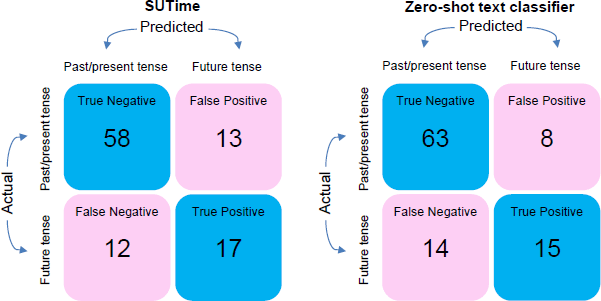
To evaluate tense-tagging accuracy, we manually assigned tense labels to 100 randomly sampled paragraphs to create a set of ‘true labels’. We then construct a confusion matrix and calculate the tense prediction accuracy for SUTime and the zero-shot classifier, respectively (Figure 8). The confusion matrix shows the performance of each algorithm (SUTime on the left and the zero-shot classifier on the right), with the rows representing the actual values and the columns showing predicted classifications. The confusion matrix shows that the two models perform similarly, with both producing high true negative rates. SUTime correctly classifies 58 out of 71 paragraphs as in the past/present tense, while the zero-shot classifier correctly classifies 63 out of 71 paragraphs. That is, both models perform well in filtering out paragraphs that are in the past or present tense. The models do not perform as well when classifying paragraphs into the future tense. SUTime performs marginally better with 17 out of 29 correct classifications, so we proceed with SUTime as our tense tagger. A comparison of the aggregate forward-looking indices is shown in Figure C1.
Sources: Authors' calculations; Reuters.
6. Firms' Price-setting Behaviour
Understanding what influences firms' price-setting behaviour is important for understanding the dynamics of the inflation process. In this section, we use panel regressions to study how firms' sentiment about final prices is associated with changes in sentiment regarding various input costs and demand and how these responses vary by industry. We also explore if there are any differences depending on whether the sentiment of the discussions about input costs and demand is increasing or decreasing, which enables us to test for evidence of price-setting asymmetries. Our estimates only represent reduced-form statistical correlations and caution should be exercised in drawing a causal interpretation from them. Caution should also be adopted when generalising our results beyond the sample of large, listed companies that are the focus here. Previous research has documented notable differences in the price-setting behaviour of larger firms compared to their smaller counterparts.[12] The insights from this exercise are complementary to those obtained from central bank surveys of firms' pricing behaviour.[13] However, compared to central bank surveys, the use of earnings calls means we can examine price-setting behaviour for a panel of firms over a long history of time and that any insights can be updated at regular intervals.
We begin by estimating the following panel regression, with the data beginning in 2007:
Here pit denotes the final price sentiment index for firm i in time period t, measured at a quarterly frequency.[14] The term is the demand sentiment index over the period 2007–2020, while is the index from 2021. Likewise, icn,it is the input cost index for input cost sentiment index . Including separate coefficients for each time period allows us to examine if there is anything different about the period since 2021 – which has been characterised by sizable supply shocks – relative to the historical sample. The regression includes firm, , and time fixed effects, . The firm fixed effects allows us to control for unobservable differences in the language used by each firm during their earnings calls. The time fixed effects control for changes in the operating environment that are common to all firms, including the effect of global supply shocks.
In Equation (4) below, we instead include separate coefficients for demand and aggregate input costs according to whether the change in sentiment was positive or negative . This allows us to examine whether price-setting sentiment changes asymmetrically in response to positive or negative changes in input costs or demand sentiment.
Finally, in Equation (5) below, the demand and input cost variables are interacted with industry dummies, , enabling us to examine variation in price-setting behaviour by industry. We also include industry-time fixed effects, , to control for changes in the operating environment that are common to all firms in a particular industry.
In all regressions standard errors are clustered at the industry level to accommodate within-industry serial correlation. All regressions are estimated using the sentiment indices from the zero-shot text classifier constructed according to Equation (2) in Section 3, with separate results presented for the overall and future-tense versions of the indices.
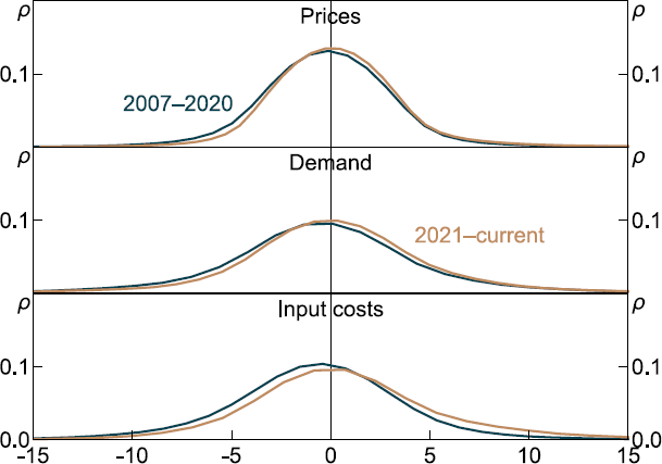
Before turning to the results, a description of the data used to estimate our regressions is provided in Table 4 below. Notably, in both the pre- and post-COVID-19 periods, there is ample within-firm variation in each of the indices to use for identifying conditional correlations between firms' final price sentiment and our various other sentiment indices. As a complement to Table 4 we can also plot the distribution of the sentiment indices for prices, demand and aggregate input costs, focusing only on changes in sentiment within firms – that is, each firm's deviation from its own average over time. Figure 9 shows there is substantial variation about the mean in both periods, with some minor right-skewness in the post-COVID-19 period. Finally, Table D1 shows cross-correlations between each of the sentiment indices, using within-firm variation only. Correlations are typically small and positive, indicating that multicollinearity is unlikely to affect the interpretation of our coefficient estimates.
| Mean | Overall standard deviation |
Within standard deviation(a) |
Min | Max | |
|---|---|---|---|---|---|
| Price07–20 | 0.6 | 3.1 | 2.6 | −28 | 29 |
| Price21–23 | 1.4 | 2.6 | 2.4 | −11 | 22 |
| Demand07–20 | 6.7 | 8.3 | 5.0 | −22 | 64 |
| Demand21–23 | 7.3 | 8.1 | 4.4 | −10 | 55 |
| Aggregate input costs07–20 | 1.6 | 4.8 | 3.9 | −29 | 37 |
| Aggregate input costs21–23 | 3.7 | 6.7 | 4.6 | −12 | 72 |
| Import costs07–20 | −0.2 | 1.5 | 1.3 | −9 | 10 |
| Import costs21–23 | −0.1 | 1.5 | 1.2 | −11 | 8 |
| Labour costs07–20 | 0.1 | 1.4 | 1.2 | −8 | 10 |
| Labour costs21–23 | 0.7 | 2.1 | 1.6 | −6 | 17 |
| Supply shortages07–20 | 0.9 | 1.7 | 1.2 | na | 20 |
| Supply shortages21–23 | 1.7 | 3.1 | 2.1 | na | 40 |
| Transport costs07–20 | 0.0 | 1.6 | 1.3 | −9 | 21 |
| Transport costs21–23 | 0.4 | 1.9 | 1.4 | −24 | 34 |
|
Note: (a) Defined as the standard deviation of the series, , where x is the topic of interest. Sources: Authors' calculations; Reuters. |
|||||
Sources: Authors' calculations; Reuters.
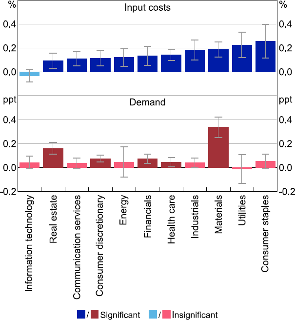
The results from estimating Equation (3) are shown in Table 5; results from estimating Equation (4) are shown in Table 6; and results from estimating Equation (5) are summarised in Figure 10. We have four key empirical findings.
First, sentiment about final prices has a significantly stronger association with sentiment about input costs compared to sentiment about demand (Table 5, column 1). The coefficients on demand and input costs shown in column 1 are statistically different at the 1 per cent level. Specifically, the results suggest a 10 percentage point increase in the share of paragraphs about demand increasing (on net) is associated with around a 1 percentage point increase in the share of paragraphs about final prices increasing (on net), whereas the same increase in references to input costs increasing (on net) is associated with a 2 percentage point increase in the share of paragraphs about final prices increasing (on net).[15] This result holds over the period 2007–2020 as well as in the post-COVID-19 period. The extra emphasis on costs is in line with messages the Reserve Bank of Australia receives from its periodic surveys of firms' pricing strategies, which indicates that the predominant pricing strategy of firms is to set prices as a mark-up on costs (Park et al 2010). It is also consistent with empirical work showing firms' expectations for their own costs are an important determinant of their price-setting behaviour – see, for example, Meyer, Parker and Sheng (2021) and Asghar, Fudurich and Voll (2023). This notwithstanding, when talking about the future, firms appear to place equal emphasis on the outlook for input costs and demand (Table 5, column 2).
Second, disaggregating input costs into selected subindices shows that the historically positive association between labour cost sentiment and final price sentiment has been weaker and statistically insignificant in the post-COVID-19 environment (Table 5, column 3). These two coefficient estimates are statistically different from each other at the 15 per cent level (t-test, p-value = 0.14). On the other hand, there has been a statistically significant increase in the association between import costs and final prices (t-test, p-value = 0.06).[16] Because we control for the impact of shocks that are common to all firms, this result cannot be attributed to the increase in global supply shocks that have occurred over the past few years. Instead, it provides tentative evidence that the pass-through of import costs to final prices may have risen recently, while the pass-through of labour costs may have fallen. This latter finding is consistent with Amiti et al (2022) for the United States, who use industry-level data to show that higher pass-through of import prices has made a significant contribution toward recent higher inflation, though they also point to higher pass-through of labour costs.
| Aggregated input costs | Disaggregated input costs | ||
|---|---|---|---|
| All tenses | Forward-looking tense | All tenses | |
| Demand07–20 | 0.085*** | 0.104*** | 0.092*** |
| Demand21–23 | 0.080*** (−0.048) |
0.089*** (−0.015) |
0.084*** (−0.009) |
| Aggregate input costs07–20 | 0.199*** | 0.106*** | |
| Aggregate input costs21–23 | 0.162*** (−0.037) |
0.089** (−0.017) |
|
| Import costs07–20 | 0.045 | ||
| Import costs21–23 | 0.165** (+0.120*) |
||
| Labour costs07–20 | 0.076* | ||
| Labour costs21–23 | −0.003 (−0.079) |
||
| Supply shortages07–20 | 0.094 | ||
| Supply shortages21–23 | 0.117** (+0.023) |
||
| Transport costs07–20 | 0.144* | ||
| Transport costs21–23 | 0.138** (−0.006) |
||
| Sample | 5,145 | 5,145 | 5,145 |
| Within R2 | 0.174 | 0.087 | 0.122 |
|
Note: Standard errors are clustered at the industry level; ***, ** and * denote statistical significance at the 1, 5 and 10 per cent levels, respectively. |
|||
Third, we uncover no pricing asymmetries with respect to whether demand sentiment has improved or deteriorated (Table 6, column 1). That is, the association with discussions about final prices is the same regardless of whether sentiment regarding demand conditions increased (indicated by in Table 6) or decreased (indicated by in Table 6). This finding appears in contrast to messages from firm-level surveys of firms' price-setting behaviour, which tend to find that falls in demand are more likely to prompt price changes – see, for example, Fabiania et al (2006). Moreover, when focusing on forward-looking indices, firms' price-setting is significantly more responsive to an improvement in demand sentiment compared to a deterioration in sentiment (t-test, p-value = 0.04) (Table 6, column 2).
By contrast, the association between input cost sentiment and final price sentiment is stronger when firms are talking about input costs increasing as opposed to decreasing (t-test, p-value = 0.06) (Table 6). This asymmetry could suggest that rising prices could remain front of mind for company executives even as input costs decline from their current high levels. Our findings in this regard are consistent with the narrative-based evidence presented in Pitschner (2020). Here the author uses archived corporate filings for a large sample of US firms to show that cost shocks only appear to matter for price increases, concluding that prices are likely to be stickier after cost decreases than they are after cost increases.
| All tenses | Forward-looking tense | |
|---|---|---|
| 0.096*** | 0.055*** | |
| 0.081*** (−0.015) |
0.107*** (+0.051**) |
|
| 0.152*** | 0.076*** | |
| 0.193*** (+0.040*) |
0.117*** (+0.041) |
|
| Sample | 4,599 | 4,599 |
| Within R2 | 0.183 | 0.097 |
| Note: Standard errors are clustered at the industry level; ***, ** and * denote statistical significance at the 1, 5 and 10 per cent levels, respectively. | ||
Finally, the results suggest that pricing behaviour differs significantly across industries, after controlling for shocks to prices that are common to all firms within an industry (Figure 10). Cost-focused strategies appear more important for the consumer staples, utilities, materials and industrial industries. Demand-focused strategies also appear important for the materials industry and to a lesser extent the real estate, consumer discretionary, financial and health care industries. These findings appear consistent with the fundamental business properties of the respective industries. For instance, prices in the consumer staples industry, which includes supermarket chains and agricultural goods and services providers, are highly exposed to supply-side shocks, such as breaks in supply chains, but the price elasticity of demand for consumer staples is typically considered to be low. On the other hand, the price elasticity of demand in the consumer discretionary industry, which includes firms providing entertainment services, tourism services, consumer durables and speciality retail is typically considered to be higher. Prices in the materials industry, which includes Australia's largest miners, are also strongly influenced by global demand factors. Taking a step back, the substantial heterogeneity by industry in these estimates illustrates that the macroeconomic impact of aggregate shocks crucially depends on which industries are particularly affected by them, a conclusion also reached by Dias et al (2015).
Note: Whiskers show 90 per cent confidence intervals.
Sources: Authors' calculations; Reuters.
7. Conclusion
This paper examines firms' price-setting behaviour using insights derived from earnings calls. We develop three sentiment indices (input costs, demand and final prices) using two different methods – one dictionary-based and one using a transformer-based large language model. We show that the signal from these indices about input costs, demand and final prices is contemporaneous with the information the Reserve Bank of Australia receives as part of its business liaison program and leads (in the sense of Granger causality) signals provided by regular firm-level surveys of business conditions. The indices for input costs and final prices also help to predict statistical measures of producer and consumer price inflation in the reference quarter, after considering the past values of both variables.
Our reduced-form analysis, uncovering conditional correlations between the sentiment of final price discussions and the sentiment of discussions about input costs and demand, allows us to draw inferences regarding firms' pricing behaviour that are relevant for understanding the dynamics of the inflation process. Our results are consistent with firms using pricing strategies that focus on a mark-up over costs. They are also consistent with firms being more reactive to rising, rather than falling, input costs. Finally, we document sizable heterogeneity in pricing behaviour across industries.
Overall, this paper shows that techniques in natural language processing can be usefully applied to understand firms' price-setting behaviour and current economic conditions more broadly. This can be a valuable tool for policymakers in assessing the inflation outlook and in understanding the dynamics of the inflation process.
We consider our paper the tip of the iceberg in terms of using large language models to examine earnings calls to better understand firm-level dynamics that are relevant for policy analysis. The capabilities of large language models are advancing rapidly. In this environment, we expect the construction of text-based macroeconomic indices derived from earnings calls to evolve in stride with these advances. For instance, future work could use alternative large language models, such as fine-tuned generative pre-trained transformative models, to annotate earnings call transcripts into topics, tone and tense. Another exciting direction of future research is to combine the firm-level textual insights extracted from the earnings calls with firm-level balance sheet and income statement data, which is readily available. This would provide a much richer panel of information to explore other interesting facets of price-setting behaviour, such as the role of competition and strategic complementarities.
Appendix A: Constructing the Dictionary-based Indices
We construct word lists for 10 subindices, shown below in Figure A1. The subindices were selected with reference to those used by the Australian Bureau of Statistics Input-Output Product Classification.
Note: Series are standardised to measure the number of standard deviations each series is from its mean value.
Sources: Authors' calculations; RBA; Reuters.
The list of keywords and qualifiers for the indices was then expanded by training a word embedding model (Word2Vec) on the earnings call corpus and adding relevant words that appeared to be missing. Overall, 70 words were used across the 10 subindices. Each word is also associated with a list of positive and negative qualifiers. To contribute to the index a keyword must appear near its qualifier (see Equation (1)). For example, the list of keywords and qualifiers for the ‘materials cost’ subindex is provided in Table A1. The same process was also used to construct the demand and final price indices.
| Keyword | Negative qualifiers | Positive qualifiers |
|---|---|---|
| equipment cost | reduce, reduction, reducing, lessening, decrease, decreasing, decreased, diminishing, diminished, lower, easing, lowering, decline, declining | pressure, higher, inflation, flow through, pass through, escalation, blowout, increasing, increased, spike, rising, increase |
| vehicle expense | reduce, reduction, reducing, lessening, decrease, decreasing, decreased, diminishing, diminished, lower, easing, lowering, decline, declining | pressure, higher, inflation, flow through, pass through, escalation, blowout, increasing, increased, spike, rising, increase |
| wood | reduce, reduction, reducing, lessening, decrease, decreasing, decreased, diminishing, diminished, lower, easing, lowering, decline, declining | pressure, higher, inflation, flow through, pass through, escalation, blowout, increasing, increased, spike, rising, increase |
| timber | reduce, reduction, reducing, lessening, decrease, decreasing, decreased, diminishing, diminished, lower, easing, lowering, decline, declining | pressure, higher, inflation, flow through, pass through, escalation, blowout, increasing, increased, spike, rising, increase |
| lumber | reduce, reduction, reducing, lessening, decrease, decreasing, decreased, diminishing, diminished, lower, easing, lowering, decline, declining | pressure, higher, inflation, flow through, pass through, escalation, blowout, increasing, increased, spike, rising, increase |
| laminate cost | reduce, reduction, reducing, lessening, decrease, decreasing, decreased, diminishing, diminished, lower, easing, lowering, decline, declining | pressure, higher, inflation, flow through, pass through, escalation, blowout, increasing, increased, spike, rising, increase |
| steel cost | reduce, reduction, reducing, lessening, decrease, decreasing, decreased, diminishing, diminished, lower, easing, lowering, decline, declining | pressure, higher, inflation, flow through, pass through, escalation, blowout, increasing, increased, spike, rising, increase |
| pipe | reduce, reduction, reducing, lessening, decrease, decreasing, decreased, diminishing, diminished, lower, easing, lowering, decline, declining | pressure, higher, inflation, flow through, pass through, escalation, blowout, increasing, increased, spike, rising, increase |
| piping | reduce, reduction, reducing, lessening, decrease, decreasing, decreased, diminishing, diminished, lower, easing, lowering, decline, declining | pressure, higher, inflation, flow through, pass through, escalation, blowout, increasing, increased, spike, rising, increase |
| aluminium | reduce, reduction, reducing, lessening, decrease, decreasing, decreased, diminishing, diminished, lower, easing, lowering, decline, declining | pressure, higher, inflation, flow through, pass through, escalation, blowout, increasing, increased, spike, rising, increase |
| metal | reduce, reduction, reducing, lessening, decrease, decreasing, decreased, diminishing, diminished, lower, easing, lowering, decline, declining | pressure, higher, inflation, flow through, pass through, escalation, blowout, increasing, increased, spike, rising, increase |
Appendix B: Matched Sample Results
| Granger causality outcome(a) | Max pairwise correlation | |||
|---|---|---|---|---|
| Input costs | earnings calls sentiment | liaison sentiment | 0.88 (liaison leads) | |
| Demand | earnings calls sentiment | → | liaison sentiment | 0.77 (contemporaneous) |
| Labour costs | earnings calls sentiment | liaison sentiment | 0.82 (contemporaneous) | |
| Prices | earnings calls sentiment | ← | liaison sentiment | 0.52 (contemporaneous) |
|
Notes: Matched over the entire sample period, not at any given point in time. (a) VARs of the form: , where yt is the measure of interest (input costs, demand, labour costs and prices), constructed using either (1) earnings calls and business liaison; (2) earnings call and surveys of firms; or (3) earnings calls and statistical measures. → and ← indicate the direction of causality with indicating bi-directional causality. |
||||
Appendix C: Tense Comparisons
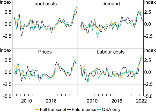
Notes: Series are standardised to measure the number of standard deviations each series is from its mean value. Rolling quarterly six-month average.
Sources: Authors' calculations; RBA; Reuters.
Appendix D: Correlations between Sentiment Indices
| Price | Demand | Aggregate input costs | Import costs | Labour costs | Supply shortages | Transport costs | |
|---|---|---|---|---|---|---|---|
| Price | 1.00 | ||||||
| Demand | 0.15 | 1.00 | |||||
| Aggregate input costs | 0.45 | 0.18 | 1.00 | ||||
| Import costs | 0.17 | 0.08 | 0.37 | 1.00 | |||
| Labour costs | 0.12 | 0.11 | 0.50 | 0.14 | 1.00 | ||
| Supply shortages | 0.24 | 0.15 | 0.64 | 0.11 | 0.23 | 1.00 | |
| Transport costs | 0.19 | 0.09 | 0.54 | 0.20 | 0.16 | 0.23 | 1.00 |
|
Sources: Authors' calculations; Reuters. |
|||||||
| Price | Demand | Aggregate input costs | Import costs | Labour costs | Supply shortages | Transport costs | |
|---|---|---|---|---|---|---|---|
| Price | 1.00 | ||||||
| Demand | 0.23 | 1.00 | |||||
| Aggregate input costs | 0.50 | 0.19 | 1.00 | ||||
| Import costs | 0.17 | 0.08 | 0.42 | 1.00 | |||
| Labour costs | 0.13 | 0.14 | 0.48 | 0.19 | 1.00 | ||
| Supply shortages | 0.17 | 0.14 | 0.53 | 0.09 | 0.21 | 1.00 | |
| Transport costs | 0.18 | 0.09 | 0.58 | 0.16 | 0.15 | 0.16 | 1.00 |
|
Sources: Authors' calculations; Reuters. |
|||||||
References
Amiti M, S Heise, F Karahan and A Şahin (2022), ‘Pass-Through of Wages and Import Prices Has Increased in the Post-COVID Period’, Federal Reserve Bank of New York Liberty Street Economics blog, 23 August, viewed 8 September 2022. Available at <https://libertystreeteconomics.newyorkfed.org/2022/08/pass-through-of-wages-and-import-prices-has-increased-in-the-post-covid-period/>.
Amiti M, O Itskhoki and J Konings (2019), ‘International Shocks, Variable Markups, and Domestic Prices’, The Review of Economic Studies, 86(6), pp 2356-2402.
Aragones E, I Gilboa, A Postlewaite and D Schmeidler (2005), ‘Fact-Free Learning’, The American Economic Review, 95(5), pp 1355-1368.
Asghar R, J Fudurich and J Voll (2023), ‘Firms’ Inflation Expectations and Price-Setting Behaviour in Canada: Evidence from a Business Survey', Bank of Canada Staff Analytical Note 2023-3.
Ash E and S Hansen (2023), ‘Text Algorithms in Economics', Centre for Economic Policy Research Discussion Paper DP18125.
Bauer MD and ET Swanson (2020), ‘An Alternative Explanation for the “Fed Information Effect”‘, Federal Reserve Bank of San Francisco Working Paper 2020-06.
Beckers B, J Hambur and T Williams (2023), ‘Estimating the Relative Contributions of Supply and Demand Drivers to Inflation in Australia’, RBA Bulletin, June.
Bloom N, TA Hassan, A Kalyani, J Lerner and A Tahoun (2021), ‘The Diffusion of Disruptive Technologies', NBER Working Paper No 28999, rev November 2021.
Bunn P, L Anayi, N Bloom, P Mizen, G Thwaites and I Yotzov (2022), ‘Firming up Price Inflation', Bank of England Staff Working Paper No 993.
Byrne D, R Goodhead, M McMahon and C Parle (2023), ‘Measuring the Temporal Dimension of Text: An Application to Policymaker Speeches’, Centre for Economic Policy Research Discussion Paper DP17931.
Chang AX and CD Manning (2012), ‘SUTime: A Library for Recognizing and Normalizing Time Expressions’, in Proceedings of the Eighth International Conference on Language Resources and Evaluation (LREC'12), Istanbul, Turkey, European Language Resources Association (ELRA), pp 3735-3740.
Dias DA, CR Marques, F Martins and JMC Santos Silva (2015), ‘Understanding Price Stickiness: Firm-Level Evidence on Price Adjustment Lags and Their Asymmetries', Oxford Bulletin of Economics and Statistics, 77(5), pp 701-718.
Dwyer J, K McLoughlin and A Walker (2022), ‘The Reserve Bank's Liaison Program Turns 21’, RBA Bulletin, September.
Fabiani S, M Druant, I Hernando, C Kwapil, B Landau, C Loupias, F Martins, T Mathä, R Sabbatini, H Stahl and A Stokman (2006), ‘What Firms’ Surveys Tell Us about Price-Setting Behavior in the Euro Area', International Journal of Central Banking, 2(3), pp 3-47.
Hassan TA, S Hollander, L van Lent and A Tahoun (2019), ‘Firm-Level Political Risk: Measurement and Effects’, The Quarterly Journal of Economics, 134(4), pp 2135–2202.
Hassan TA, J Schreger, M Schwedeler and A Tahoun (2021), ‘Sources and Transmission of Country Risk’, NBER Working Paper No 29526.
Jamilov R, H Rey and A Tahoun (2021), ‘The Anatomy of Cyber Risk’, NBER Working Paper No 28906.
King G, P Lam and ME Roberts (2017), ‘Computer-Assisted Keyword and Document Set Discovery from Unstructured Text’, American Journal of Political Science, 61(4), pp 971–988.
Lewis M, Y Liu, N Goyal, M Ghazvininejad, A Mohamed, O Levy, V Stoyanov and L Zettlemoyer (2019), ‘BART: Denoising Sequence-to-Sequence Pre-training for Natural Language Generation, Translation, and Comprehension’, Unpublished manuscript, 29 October. Available at <https://doi.org/10.48550/arXiv.1910.13461>.
Meyer BH, NB Parker and XS Sheng (2021), ‘Unit Cost Expectations and Uncertainty: Firms’ Perspectives on Inflation', Federal Reserve Bank of Atlanta Working Paper 2021-12a, rev December 2021.
O'Neill L, N Anantharama, W Buntine and SD Angus (2021), ‘Quantitative Discourse Analysis at Scale – AI, NLP and the Transformer Revolution’, SoDa Laboratories Working Paper Series No 2021-12.
Park A, V Rayner and P D'Arcy (2010), ‘Price-Setting Behaviour – Insights from Australian Firms’, RBA Bulletin, June, pp 7–14.
Peltzman S (2000), ‘Prices Rise Faster than They Fall, Journal of Political Economy, 108(3), pp 466–502.
Pitschner S (2020), ‘How Do Firms Set Prices? Narrative Evidence from Corporate Filings’, European Economic Review, 124, Article 103406.
Rees DM (2020), ‘What Comes Next?’, BIS Working Paper No 898.
Sautner Z, L van Lent, G Vilkov and R Zhang (2023), ‘Firm-Level Climate Change Exposure’, The Journal of Finance, 78(3), pp 1449–1498.
Toda HY and T Yamamoto (1995), ‘Statistical Inference in Vector Autoregressions with Possibly Integrated Processes’, Journal of Econometrics, 66(1–2), pp 225–250.
Wigglesworth R (2022), ‘Listen to Analysts, Not Management’, FT Alphaville blog, 4 October, viewed 4 October 2022. Available at <https://www.ft.com/content/f83e8f96-6d70-4265-83ac-7cf17c2a7463>.
Yin W, J Hay and D Roth (2019), ‘Benchmarking Zero-shot Text Classification: Datasets, Evaluation and Entailment Approach’, Unpublished manuscript, 31 August. Available at <https://doi.org/10.48550/arXiv.1909.00161>.
Young HL, A Monken, F Haberkorn and E Van Leemput (2021), ‘Effects of Supply Chain Bottlenecks on Prices Using Textual Analysis’, Board of Governors of the Federal Reserve System, FEDS Notes, 3 December.
Acknowledgements
This paper has benefited from input from Michael McMahon, John Simon, Jonathan Hambur, Susan Black, Yad Haidari, Thomas Williams, Finn Lattimore and seminar participants at the Australian Conference of Economists 2023, the RBA–APRA Business Coding Knowledge Sharing Session and the e61/MQBS Big Data Workshop. Many thanks also to Harry Braithwaite for his assistance in the early stages of this work. The views expressed in this paper are those of the authors and should not be attributed to the Reserve Bank of Australia. Any errors are the sole responsibility of the authors.
Footnotes
See Beckers, Hambur and Williams (2023) for an estimate of the relative contribution of supply- and demand-side drivers to inflation in Australia. [1]
All of the code underlying our analysis of the earnings calls, index construction and empirical results is available in the online Supplementary Information. [2]
We used judgement to select the 70 per cent threshold after doing a number of ‘spot checks’ of the resulting classifications. An alternative approach is to create each topic-specific index by weighting each paragraph by its topic-specific probability. We use a threshold because our first priority is to minimise false positives, recognising this comes at the cost of not utilising all of the available textual information. Regardless, at an aggregate level, the results from both approaches (using a threshold or probability weighting) are very similar. [3]
This model is available on Huggingface (see <https://huggingface.co>). Huggingface is an open-source library for NLP providing a wide variety of transformers and models for text classification, text generation, sentiment analysis, named entity recognition and more. [4]
The pre-training does not include any earnings call transcripts. [5]
Lewis et al (2019) corrupt text snippets in the following ways: (1) token masking, where random words are replaced with blanks; (2) token deletion, the same as (1), but the model must decide which positions are missing inputs; (3) text infilling, where spans of text are filled with a blank; (4) sentence permutation, where sentences in a text snippet are randomly shuffled; and (5) document rotation, where a random word from the text snippet is cut and pasted into the opening position of the text snippet. [6]
Other large language models would be more suitable for other tasks. For instance, while ChatGPT's underlying generative pre-trained transformer-based models have the same underlying architecture, they are trained to generate coherent and contextually relevant text, making them more suitable for generating conversational responses. [7]
It is important to note here that we are only trying to establish if information taken from earnings calls are relevant for assessing current economic conditions. We are not examining if there is any information about the statistical measures over and above that contained in other indicators of current economic conditions. That is, we are not concerned with examining if the information extracted from earnings calls is useful for making marginal improvements to nowcasts of these variables. [8]
These correlations are still strong, albeit a little weaker, if we exclude the period since 2021. [9]
In comparing earnings calls to business liaison, we also ran Granger causality tests using a matched sample of 180 firms appearing in both the earnings call sample and the Reserve Bank of Australia's business liaison program. To record a match, firms had to appear only once in both samples – we did not require that firms also appear in the same time period. The results are like those reported for the full sample, although correlations are weaker (see Appendix B). [10]
We also experimented with a third (and ultimately inferior) approach, which was to restrict our analysis to only the Q&A sections of the transcripts. Previous work has shown that analysts' questions have more forward-looking information content than managements' remarks, possibly because they are more interested in the outlook and less likely to put a positive spin on things (Wigglesworth 2022). [11]
For example, Amiti, Itskhoki and Konings (2019) find that small firms exhibit complete cost pass-through whereas the pass-through of larger firms is only around 50 per cent. [12]
For example, Bunn et al (2022) for a Bank of England survey; Fabiania et al (2006) for a European Central Bank survey; and Park et al (2010) for a survey by the Reserve Bank of Australia. [13]
The methodology used here is broadly similar to that used in Young et al (2021). [14]
The relativity in these impacts is similar if we standardise the variables and examine the association to a one standard deviation change. [15]
One potential explanation for the results about labour and import costs is that executives have limited speaking time and so only focus on some issues (e.g. import costs) at the expense of other issues (e.g. labour costs). If this was the case, there would be a negative within-firm correlation between references to our topics of interest. Instead, Table D2 shows that all of the correlations are positive. [16]