Bulletin – March 2019 Australian Economy Wealth and Consumption
- Download 644KB

Abstract
Do households consume more when their wealth increases? Our research identifies a positive and stable relationship between household wealth and consumption, largely reflecting changes in spending on motor vehicles, durable goods and other discretionary spending. Increases in household wealth supported household spending between 2013 and 2017, when growth in disposable income was weak. Similarly, declines in household wealth typically weigh on consumption. However, a decline in household wealth is less likely to coincide with weaker consumption growth if it occurs at a time when the labour market is strong and household income growth is firm.
Introduction
Over the past decade, Australian households' wealth has changed significantly. An important consideration in assessing the macroeconomic outlook is how these changes in wealth affect household consumption. Because consumption accounts for a large share of aggregate demand, the consumption response to changes in wealth can also affect economic activity more broadly.
In this article we revisit the relationship between household wealth and consumption. We first document recent trends in the two variables. We then provide updated estimates of the empirical relationship between consumption and wealth, and compare these estimates to other studies in Australia and overseas. Finally, we use the RBA's macroeconomic model, MARTIN, to explore the broader macroeconomic consequences of changes in household wealth.
Recent Trends in Household Wealth and Consumption
Household wealth is measured as the household sector's assets minus its liabilities. Household assets comprise financial assets, which include bank deposits, direct equity holdings and superannuation balances, and non-financial assets, which include housing and durable items such as motor vehicles. The household sector's liabilities are largely made up of residential mortgages, but also include items such as credit card debt and personal loans.
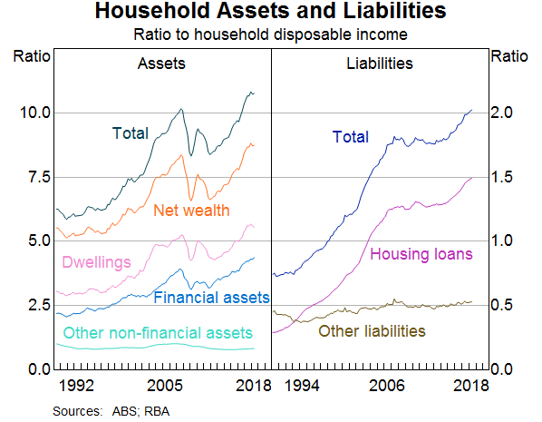
Household wealth has grown much faster than household income over recent decades (Graph 1). This is largely because of increases in the value of household assets, which have grown from around six times household disposable income in the early 1990s to around eleven times currently. Household liabilities have also grown faster than household income, although by less than household assets. The rate of growth of household wealth varies greatly from year to year and on several occasions, such as during the Global Financial Crisis, the value of household wealth has declined. After increasing by around 60 per cent between 2013 and 2017, growth in household wealth has slowed recently because of falling housing prices.
Household consumption growth is much more stable than wealth from year to year. After averaging around 5 per cent in year-ended terms between the early 1990s and mid 2000s, the pace of household consumption growth has eased to a bit above 2½ per cent in recent years (Graph 2). Modest growth in consumption alongside fast growth in wealth could be taken to mean that changes in wealth have little effect on consumption. In making that judgement, however, it is important to account for other factors that influence consumption growth, such as household income. As the top panel of Graph 2 shows, consumption and income tend to grow at similar rates over time, although income growth is more volatile. Between 2013 and 2017, when household wealth was increasing rapidly, household income growth was low.
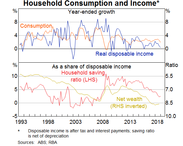
The difference between household consumption and income is reflected in the household saving ratio.[1] Changes in the saving ratio point to a positive relationship between household wealth and consumption. When household wealth grows strongly, consumption typically grows faster than household income and the saving ratio tends to decline. For example, between the 1990s and early 2000s, and again between 2013 and 2017, when household wealth was increasing rapidly, the household saving ratio fell. The opposite typically occurs when household wealth falls. For instance, during the Global Financial Crisis, when household wealth declined, the saving ratio increased (although this had already started some years earlier for other reasons).
The patterns highlighted in Graph 2 are consistent with the idea that strong growth in household wealth supported consumption growth in recent years, while, at the same time, weak growth in household income meant that consumption grew more slowly than it did in the 1990s and early 2000s. These relationships may not be causal, however, as other factors influencing both wealth and consumption may drive the correlation between the two variables. In addition, aggregate trends do not tell us how large the effects of changes in household wealth on consumption are. We address these issues in the analysis below by studying the relationship between household wealth and consumption in each Australian state.
Box: What Are Wealth Effects?
The response of consumption to unexpected changes in wealth is referred to as the ‘wealth effect’. Wealth effects can occur for a number of reasons. ‘Traditional’ wealth effects occur because, when wealth unexpectedly increases, households have more resources to support consumption over their lifetime. In simple models, where households face no transaction costs or collateral constraints on borrowing, the consumption response to a change in wealth will depend only on how much households want to smooth consumption over time and how persistent they expect the change in wealth to be (Friedman (1957), Ando and Modigliani (1963)).
In reality, the size of traditional wealth effects is likely to vary between different sources of wealth. One reason for this is because of differences in the cost of buying and selling different types of assets (Kaplan and Violante 2014). For example, it is easier to consume gains in the value of directly held equities than it is to consume gains in the value of housing or superannuation accounts. Traditional wealth effects from housing wealth could also be smaller than from other sources of wealth because housing wealth often increases at the same time as it becomes more expensive to rent or buy a home (Sinai and Souleles (2005), Buiter (2008)). However, aggregate wealth effects from housing may still exist if home owners, who see an immediate increase in their wealth, adjust their consumption by more than future home buyers and renters, for whom the increased costs of living lie in the distant future (Berger et al 2018).
Changes in wealth may also be associated with changes in consumption for other reasons. For example, an increase in household wealth may make it easier for households to borrow in order to smooth cyclical variations in their income (Campbell and Cocco (2007), Iacoviello and Neri (2010)). Expectations of improved economic conditions could lead to a rise in the value of shares and other financial assets, while at the same time encouraging households to consume more in anticipation of higher income in the future. Financial liberalisation in Australia increased the borrowing capacity of consumers, which may have also led to an increase in consumption and asset prices. In addition, rising housing prices are often associated with a larger number of housing transactions. Because households typically purchase housing-related goods and services in the months before and after a home purchase, an increase in housing transactions is likely to be associated with increased consumption (Benmelech, Guren and Melzer 2017).
Although it is difficult to isolate the precise mechanisms through which wealth affects consumption, the observed relationship between consumption and wealth is reliable and consistent. We can therefore use it to help form a view about the state of the economy.
How Much Does Consumption Respond to Changes in Wealth?
In this section, we first estimate the response of consumption to changes in financial and non-financial wealth. We then discuss which components of consumption respond most to changes in household wealth and compare our estimates to others in the literature.
Updated estimates for Australia
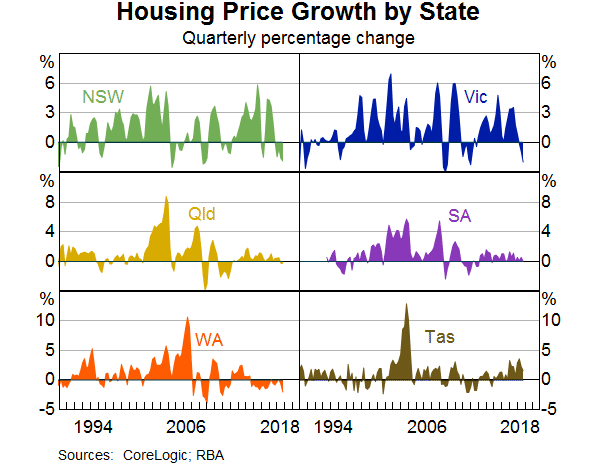
At an aggregate level, components of wealth often move together, which makes it hard to disentangle their individual effects on consumption. We follow the approach described in Case, Quigley and Shiller (2013) and Dvornak and Kohler (2007), and estimate the relationship between consumption, stock market wealth and housing wealth at a state level.[2] Each state's housing market is geographically distinct and is affected by region-specific shocks as well as national macroeconomic fluctuations (Graph 3). In contrast, movements in stock market wealth are more synchronised across the states because the value of a household's financial assets is typically unaffected by its state of residence. This geographical variability helps us to distinguish between the effects of changes in stock market and housing wealth on consumption.
Our baseline model estimates the relationship between consumption, stock market wealth, housing wealth and household income in each state in a given quarter (see Appendix A for details). We control for income because factors that increase income growth are also likely to raise household wealth and consumption. We estimate the model using data in log levels. This provides us with estimates of the long-run elasticities – the percentage change in consumption following a permanent one per cent change in wealth or income.
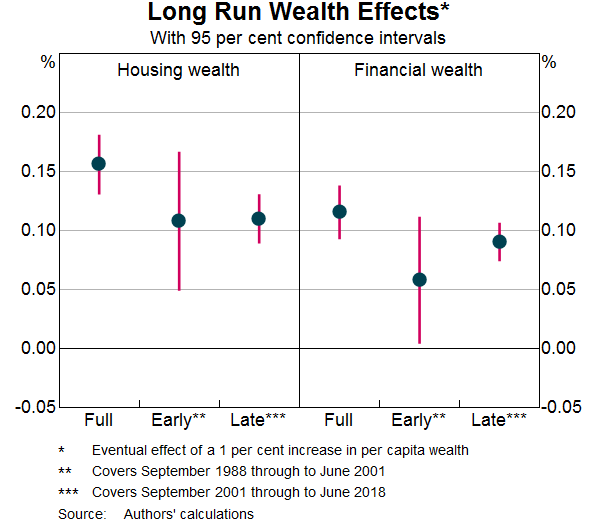
Graph 4 shows our main results. The left panel shows the estimated elasticity of consumption with respect to housing wealth, while the right panel shows the estimated elasticity with respect to stock market wealth. In each panel, the first dot shows the point estimate – or most likely value – of the elasticity over our full sample, which spans 1988Q3 to 2018Q3. The vertical lines shows 95 per cent confidence intervals, which convey a sense of the uncertainty around the point estimates. In each panel, the second and third dots show results when we split the sample in two and separately analyse each sub-sample.[3] This gives us a sense of whether wealth effects have changed over time.
The results from the full sample estimation suggest that a one per cent increase in the value of housing wealth will lead to a 0.16 per cent increase in the long-run level of consumption, while a one per cent increase in stock market wealth will raise consumption by 0.12 per cent.[4] The estimated coefficients do not differ substantially between the two sub-samples, which suggests that wealth effects are as large today as they were in the past.
Our baseline results show the relationship between the levels of consumption, income and wealth. However, estimates of relationships in levels can be biased if the model specification does not control for other long-run trends that may affect both wealth and consumption. To address this issue, we also estimate the relationship between the growth rate of consumption and those of income and wealth. As well as being more robust to omitted long-run trends, this exercise gives us a sense of how quickly consumption responds to changes in wealth. However, it may underestimate the total response if consumption adjusts slowly to changes in wealth or income.
Graph 5 shows the results of this approach. The graph summarises the response of consumption to each component of wealth after two quarters. As before, in each graph the dots represent the point estimates for each regression, while the vertical lines show 95 per cent confidence intervals.
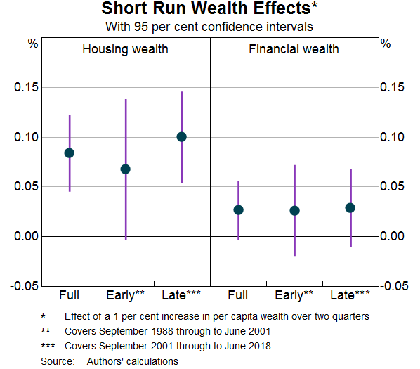
The results indicate that consumption responds quickly to changes in housing wealth. A one per cent increase in housing wealth raises consumption by 0.08 per cent over two quarters, representing around half of the long-run response shown in Graph 4. As before, the estimates are consistent across early and late sub-samples. In contrast, the response to changes in stock market wealth is small and statistically insignificant. Although our baseline results in Graph 4 suggest that changes in stock market wealth will ultimately affect consumption, those effects do not tend to occur in the first six months after the change.[5]
Which components of consumption respond most?
We re-estimate the model used in Graph 5 using more disaggregated consumption data to determine which components of consumption respond most to changes in housing wealth.[6] Graph 6 shows the results of this exercise. Once again, the dots show the estimated elasticity of each component of consumption with respect to housing wealth, while the vertical lines show 95 per cent confidence intervals around these estimates. To give an indication of how important each component of consumption is to the aggregate effect, the bars show the share of each component in aggregate consumption.
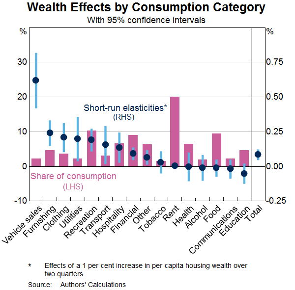
The components of consumption that respond most to changes in wealth are typically durable goods, such as motor vehicles and household furnishings. The responsiveness of motor vehicles is particularly large – a one per cent increase in housing wealth raises expenditure on motor vehicles by 0.6 per cent.[7] Many of the other expenditure categories that show a large response are discretionary items, such as recreation. In contrast, expenditure on less discretionary items – such as food, rent and education – appears to be insensitive to changes in housing wealth. Several of these components account for a large share of aggregate consumption expenditure. This helps to reconcile the large elasticities for categories like vehicle sales and home furnishings with the smaller aggregate elasticities reported in Graphs 4 and 5.
Elasticities or marginal propensities to consume?
So far, we have described wealth effects in terms of elasticities – the percentage change in consumption following a one per cent change in each component of wealth. An alternative way of expressing wealth effects is in terms of marginal propensities to consume, or MPCs. An MPC describes the dollar change in consumption to a one dollar change in wealth. We can convert our results into MPCs by multiplying the estimated elasticities in Graph 4 by the average ratio of consumption to housing wealth or stock market wealth over each sample, using the formula:
Although the estimated elasticities for changes in stock market wealth and housing wealth are similar, the estimated MPC for stock market wealth is much larger: a one dollar increase in stock market wealth raises annual consumption by about 15 cents, whereas a one dollar increase in housing wealth raises annual consumption by about 3 cents. When we repeat this exercise for our two sub-periods, we find that the MPC out of housing wealth is lower in the late sample than it was in the early sample.
We can reconcile stable elasticities with declining MPCs by the fact that the value of housing wealth has increased much faster than consumption over recent decades. The estimates in Graph 4 show that the percentage change in consumption following a given percentage change in housing wealth has been stable over time. However, because the value of housing wealth is much larger today than it was in the past, a one dollar increase in housing wealth represents a much smaller percentage change in wealth today. Aggregate consumption has also grown over this time, but not by as much. Hence, the estimated MPC out of housing wealth has declined. The fact that the value of housing wealth exceeds the value of stock market wealth also explains why the estimated MPC out of stock market wealth is larger than the MPC out of housing wealth, even though the two elasticities are similar.
Whether an elasticity or an MPC is the most appropriate measure of how wealth affects consumption depends on the question one is asking. When assessing the macroeconomic consequences of changes in wealth, one is generally interested in the percentage change in aggregate consumption following a percentage change in a component of wealth. For that purpose, elasticity estimates are most appropriate.
How do these results compare to other estimates?
Other researchers, both in Australia and overseas, have studied how much consumption responds to changes in wealth. Comparing our results to others in the literature, many of which were constructed using different data sources and methodologies to our estimates, provides another indication of the uncertainty surrounding the size of wealth effects. Because more recent studies have access to more data than earlier studies, this exercise can also give a sense of whether the estimates have changed over time.
Graph 7 compares estimated elasticities of consumption with respect to housing wealth for Australia and the US.[8] Each dot represents a study and is placed in order of its publication date. Most studies point to an elasticity between 0.1 and 0.2, which is consistent with our results in Graphs 4 and 5. Differences in housing market institutions and housing price developments between the US and Australia do not seem to cause systematic differences in the estimated elasticities between the two countries. Moreover, the similarity between earlier and more recent estimates suggests that the elasticities have been stable over time.
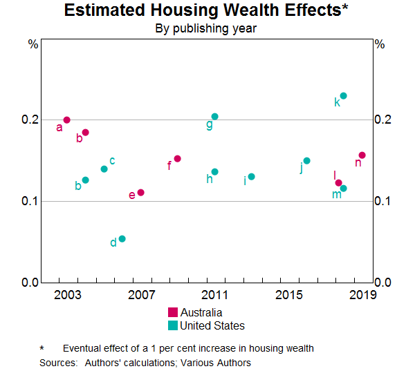
If we reproduce Graph 7 using estimated MPCs rather than elasticities, we observe much greater variation between results, as well as persistent differences across countries and time. In general, studies that work with US data report larger MPCs out of housing wealth than Australian studies. This reflects the fact that the value of housing wealth is larger relative to consumption expenditure in Australia than it is in the US. MPC estimates also appear to have been declining over time. We view the consistency in elasticity estimates across studies and wide variation in MPC estimates as a further reason why one should rely on elasticity estimates to analyse the macroeconomic consequences of changes in household wealth.[9]
Macroeconomic Consequences of Recent Changes in Household Wealth
We use MARTIN, the RBA's macroeconometric model, to assess the macroeconomic implications of changes in household wealth.[10] We first examine the extent to which increases in household wealth between 2013 and 2017 supported consumption growth. We then estimate the potential consequences of a prolonged fall in housing prices.
In MARTIN, the long-run level of consumption is determined by household disposable income, net wealth and the level of real interest rates. In the short run, changes in income, wealth and the unemployment rate as well as the economy's long-run trend growth rate also influence consumption. The model's estimate of the long-run elasticity of consumption with respect to net wealth is 0.17, which is consistent with the estimates in Graph 4.
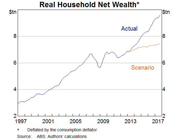
To explore how much household wealth supported consumption in recent years, we simulate the model so that it exactly replicates the driving forces, or ‘shocks’, that influenced the Australian economy over the past 20 years for all variables except for net wealth, which we constrain to grow at the same rate as household disposable income from 2013 to 2017. Year-ended growth in net wealth is about 5 percentage points lower on average in the scenario than it was in the data (Graph 8). By comparing the values of macroeconomic variables in the scenario to their values in the data, we can infer how much the growth in net wealth contributed to macroeconomic outcomes.
We identify the implications of lower wealth for household consumption in two steps. In the first, we hold all variables, except for consumption and wealth, at their actual values. This reveals the direct effects of lower wealth on consumption. Average year-ended consumption growth is about ¾ of a percentage point lower in the scenario (Graph 9). With income unchanged, this implies a household saving ratio of about 6.5 per cent at the end of 2017 as opposed to its actual value of 4.1 per cent.
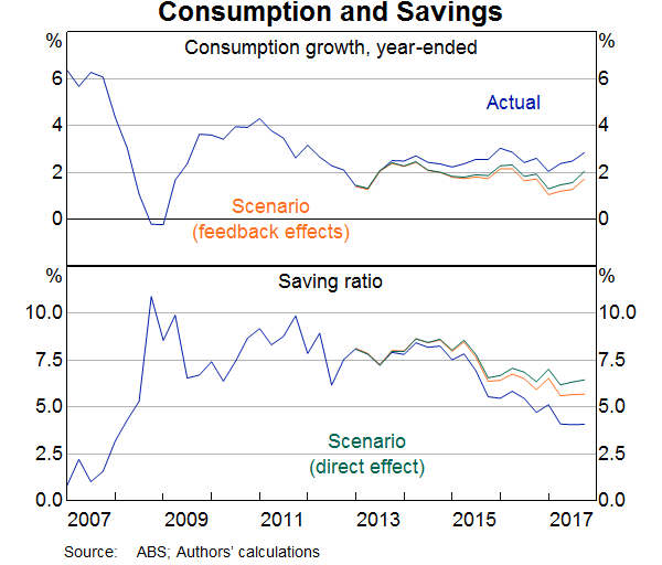
In the second step, we allow the rest of the model to respond. This accounts for feedback effects from other variables and reveals the full effect of lower wealth on consumption according to the MARTIN model. As Graph 9 shows, the direct effects initially dominate, but over time the indirect effects become important. By the end of 2017 they account for around a quarter of the 1.2 percentage point decrease in year-ended consumption growth. The household saving ratio is also lower than in the case with only direct effects, because household income falls by more than consumption.
Our second exercise examines the effects of a prolonged fall in housing prices. Specifically, we consider a 10 per cent fall in national housing prices that persists for five years. It should be noted that such a prolonged downturn is outside the usual range of experience in Australia, and therefore the estimated relationships in MARTIN, which capture the average of past experience, might be less reliable. We first discuss results assuming that the cash rate remains fixed at its initial level, which allows us to isolate the effects of lower housing prices independently of other economic developments. This turns out to have a modest contractionary effect on economic activity. We then show how the results change when we allow the cash rate to respond, the arguments for which would be stronger if the decline in housing prices were to coincide with a broader deterioration in economic conditions. Graphs 10 and 11 show the results of the scenarios, with all variables expressed as deviations from a baseline where housing prices are stable.
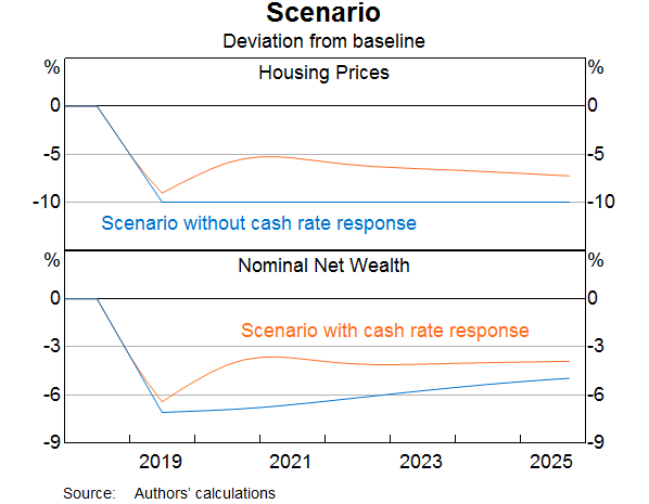
A fall in housing prices affects the economy in several ways. As well as lowering net wealth and household consumption, lower housing prices also reduce incentives to build new housing. The decline in household consumption and residential construction activity reduce aggregate demand, which leads to lower business investment. The net effect of these developments is that economic activity expands more slowly than would have been the case if housing prices did not fall; the level of GDP is 1.2 per cent below its baseline level after three years and remains low for some time. The decline in economic activity lowers the demand for labour and causes an increase in the unemployment rate, which rises by 0.4 percentage points, assuming that the estimated relationships in the model are correct (Graph 11). To put the results in context, this increase in the unemployment rate is around one quarter of the rise in the trend unemployment rate that occurred in 2008–09 during the Global Financial Crisis.
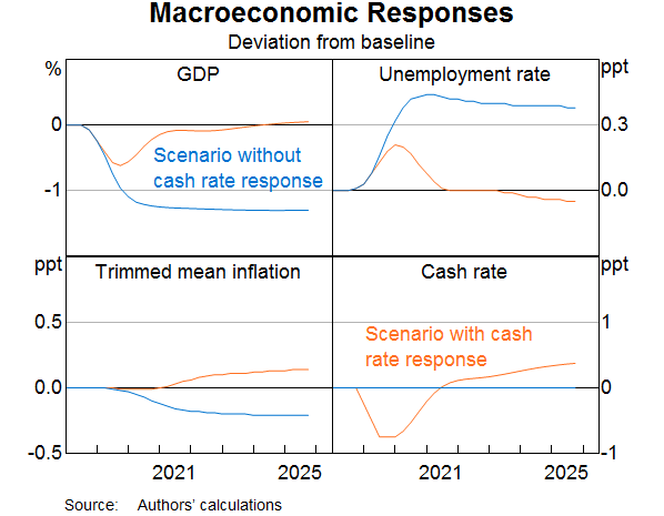
Changes in housing prices rarely occur in isolation. The net effect of a fall in housing prices that occurs when broader macroeconomic conditions are positive – for example, if the unemployment rate is falling and the global economy is expanding at a solid pace – might be only a small slowdown in the pace of economic activity. However, if the same fall in housing prices occurred alongside a broader slowdown in economic conditions, this could add to any case for an easing of monetary policy coming from the broader slowdown. As an example of a monetary policy response that could largely offset the effect of lower housing prices, we consider a hypothetical cash rate profile illustrated with the orange line in Graph 11.
The macroeconomic consequences of falling housing prices are smaller and less sustained when monetary policy responds. In this case, the decline in the level of GDP is about half as large as when the cash rate is constant, and GDP returns to its baseline level after two years. The increase in the unemployment rate is also much smaller and less persistent.
With lower interest rates, housing prices do not fall by as much as they do when the cash rate is held constant. Nonetheless, housing prices remain below their baseline level. This is because monetary policy targets inflation and full employment, not asset prices. Lower interest rates stimulate the economy in part through the housing market. But other mechanisms, such as easier cash flow constraints on households and a depreciation of the exchange rate, are also important. As a result, monetary policy can stabilise economic activity and inflation without necessarily returning housing prices to their initial level.
More generally, the exact size and timing of any change in interest rates in response to a fall in housing prices would depend on a range of factors, including the other forces affecting the economy. As mentioned previously, a fall in housing prices would have fewer negative consequences if it was offset by other developments which meant that the overall economic outlook was positive and the unemployment rate was falling. Also relevant are the expectations of households and businesses: if they continue to expect strong growth and inflation in line with the target in the longer term, despite the fall in housing prices, interest rates may not need to be reduced as much to offset the effect of that price fall. Although MARTIN cannot capture these features, they may be relevant in the Australian context.
Conclusion
When wealth increases, Australian households consume more. Spending on durable goods, like motor vehicles, and discretionary goods, such as recreation, appears to be most responsive to changes in household wealth, although many categories of consumption expenditure appear to grow more quickly when wealth increases. The positive relationship between consumption and wealth is particularly robust for housing wealth and has been stable over time.
Our simulation results suggest that strong growth in household wealth played a meaningful role in supporting consumption growth between 2013 and 2017. However, wealth is only one of the factors determining aggregate consumption growth. In recent years, rapid increases in household wealth have coincided with comparatively modest growth in household consumption, because income growth was weak. Similarly, declines in household wealth may not correspond to lower consumption growth if other factors, such as strong employment and income growth and accommodative monetary policy, are providing support.
Appendix A: Estimating the Relationship between Consumption and Wealth
Our baseline regression to assess the relationship between consumption and wealth is:
Where is household consumption in state at time is stock market wealth, is housing wealth and is compensation of employees, which accounts for the bulk of household income. All variables are in real per capita terms. We include state-level fixed effects to control for factors like the age structure of the population, which might cause some states to consume more than others relative to their income and wealth. Fixed effects will also control for systematic error in the measurement of the dependent variables. We assume, however, that the proportional response of consumption to changes in income or wealth is the same in each state.[11]
Table A1 shows our main results. The first three columns show the estimated elasticities of consumption with respect to stock market wealth, housing wealth and income over different sample periods. The first column shows estimates over the full sample, which spans 1988Q3 to 2018Q2. The second and third columns show results when we split the sample in two and separately analyse each sub-sample.
The results from the full sample estimation suggest that a one per cent increase in the value of equity or housing wealth will lead to a 0.12–0.16 per cent increase in the long-run level of consumption. The estimated coefficients on wealth over the two sub-samples are similar, suggesting that wealth effects are as large today as they were in the past.
The last column in Table A1 shows the implied estimates of the marginal propensity to consume out of income and wealth from our full sample estimates. We derive these by multiplying our full sample elasticities by the average ratio of annual consumption to stock market wealth, housing wealth or labour income over our full sample.
| Variable | Elasticity | Marginal Propensity to Consume | ||
|---|---|---|---|---|
| Full sample 1988Q3–2018Q2 |
Early sample 1988Q3–2001Q2 |
Late sample 2001Q3–2018Q2 |
Full sample 1988Q3–2018Q2 |
|
| Stock market wealth | 0.12** (0.01) |
0.06 (0.03) |
0.09** (0.02) |
15 |
| Housing wealth | 0.16** (0.01) |
0.11** (0.03) |
0.11** (0.01) |
3 |
| Disposable income | 0.45** (0.01) |
0.84** (0.06) |
0.50** (0.02) |
54 |
| No. Observations | 672 | 264 | 408 | |
| No. Groups | 6 | 6 | 6 | |
|
* and ** denote significance at the 10 and 5 per cent level. Standard errors are in parentheses. Sources: Authors' calculations. |
||||
As an alternative to our levels specification, we also estimate the relationship between the growth rates of consumption, income and wealth:
Where is the log change in consumption (approximately equal to its growth rate), which is regressed against the current and previous growth rates of income and wealth, in addition to state fixed effects.[12] As well as being more robust to omitted long-run trends, this exercise gives us a sense of how quickly consumption responds to changes in wealth. However, it may underestimate the total response if consumption adjusts slowly to changes in wealth or income.
Table A2 shows the results of this approach. To ease interpretation, we have summed the response of consumption to each of the variables after two quarters.
| Full Sample(a) 1988Q3–2018Q2 | |
|---|---|
| Stock market wealth | 0.03 |
| Housing wealth | 0.08** |
| Income | 0.10** |
| Lagged consumption | 0.06 |
| State fixed effects | Y |
|
(a) Estimate of the sum of the coefficients. ** denotes significance at the 5 per cent level using a Wald test for joint significance. Sources: Authors' calculations |
|
In addition to the specifications described above, we have also conducted a number of additional robustness checks on our baseline estimation results. For the first two checks, we included additional explanatory variables – housing turnover and household credit – in addition to wealth and income. For the third robustness check, we included time fixed effects. This controls for omitted variables, like the stance of monetary policy, that are common to all states in a given time period.
The specific models that we estimated were:
Where in addition to the variables described above, is the housing turnover rate, is housing credit and is a time fixed effect. Because state-level dwelling turnover and housing credit data is not available before 2004, we estimate Equations A3 and A4 on a restricted sample. We omitted stock market wealth from Equation A5 because of the lack of variation in changes in stock market wealth across states. Table A3 shows the results of these exercises.
| (1) Dwelling turnover 2004Q1–2017Q4 |
(2) Housing Credit 2004Q1–2017Q4 |
(3) Time Fixed Effects 1988Q3–2018Q2 |
|
|---|---|---|---|
| Stock market wealth | 0.02 | 0.01 | na |
| Housing wealth | 0.07** | 0.09** | 0.07** |
| Income | 0.17** | 0.15** | 0.02 |
| Lagged consumption | −0.03 | −0.05 | 0.03 |
| Dwelling turnover rate(b) | 0.60* | ||
| Housing credit | 0.16** | ||
| State fixed effects | Y | Y | Y |
| Time fixed effects | Y | ||
|
(a) Estimate of the sum of the coefficients. ** and * denote significance
at the 5 per cent and 10 per cent level respectively using a Wald test
for joint significance. Sources: Authors' calculations |
|||
The results in Table A3 indicate that both turnover and credit tend to have a positive effect on consumption, which suggests that they can account for part of the transmission of changes in household wealth to consumption. However, in both cases, the coefficient on housing wealth remains largely unchanged from our baseline results, after one accounts for the restricted sample. When we include time fixed effects, the estimated response of consumption to changes in housing wealth is marginally smaller than in our baseline specification, although it remains statistically significant. Overall, our results are robust to these alternative specifications.
Footnotes
The authors work in the Economic Analysis Department and would like to thank Penelope Smith, Tom Rosewall and Peter Tulip for their comments and suggestions. [*]
As well as consumption and income, the household saving ratio also takes into account consumption of fixed capital, which is a measure of depreciation on households' assets. However, because this latter component tends to be fairly stable from year to year, changes in the household saving ratio are driven almost entirely by growth in consumption and income. [1]
We focus on stock market wealth and housing wealth because data are readily available and these components account for most short-run changes in household wealth. [2]
Our two samples span 1988–2001 and 2001–18. The early sample allows us to compare our results to those published in Dvornak and Kohler (2007), which is the standard reference for wealth effects in Australia. Splitting the sample in 2004, which makes the early and late samples of equal length, generates similar results. [3]
These elasticities show the effect of a one per cent change in gross housing or stock market wealth. Elasticities with respect to a change in net housing or stock market wealth are around 20 per cent smaller. [4]
It could be that because stock prices exhibit a large amount of short-run volatility, households wait to see how persistent changes are before adjusting their consumption to changes in the value of their stock market wealth. However, in light of the results in Graph 5, we can be less confident about the consumption responses to changes in financial wealth, particularly in the short run, than we are about the consumption responses to non-financial wealth. [5]
We focus on housing wealth because it is the largest component of household wealth. [6]
This elasticity is consistent with the evidence presented in Gillitzer and Wang (2016), who report an elasticity of motor vehicle registrations with respect to housing prices of 0.5 per cent, although their estimate for total consumption is smaller than ours. [7]
Sources: (a) Tan and Voss (2003), (b) Ludvig and Slok (2004), (c) Case, Quigley and Shiller (2005), (d) Juster et al (2006), (e) Slacalek (2009), (f) Kohler and Dvornak (2007), (g) Carroll, Otsuka and Slacalek (2011),(h) Iacoviello (2011), (i) Case, Quigley and Shiller (2013), (j) Kaplan, Mitman and Violante (2016), (k) Berger et al (2018), (l) Cusbert and Kendall (2018), (m) Guren et al (2018), and (n) May, Nodari and Rees (2019). [8]
In particular, it may be better to convert an elasticity estimate into an MPC using the current value of housing wealth and consumption, rather than rely on an MPC estimate calculated in the past. [9]
An advantage of using MARTIN is that it accounts for feedback between consumption and other macroeconomic variables. For example, an increase in consumption will boost aggregate demand, leading to increased employment and faster wages growth. This, in turn, will raise household income, causing further increases in consumption. See Cusbert and Kendall (2018) for a description of MARTIN. [10]
Our model implicitly assigns an equal weight to each state. However, the results are almost identical if we were instead to weight each state by its population share. [11]
We are unable to include time fixed effects in the baseline specification because there is insufficient cross-state variation in stock market wealth. [12]
References
Ando A and F Modigliani (1963), ‘The ‘Life-Cycle’ Hypothesis of Saving: Aggregate Implications and Tests', American Economic Review, 53(1), pp 55–84.
Benmelech E, A Guren and BT Melzer (2017), ‘Making the House a Home: The Stimulative Effect of Home Purchases of Consumption and Investment’, NBER Working Paper 23570.
Berger D, V Guerrieri, G Lorenzoni and J Vavra (2018), ‘House Prices and Consumer Spending’, Review of Economic Studies, 85(3), pp 1502–1542.
Buiter WH (2008), ‘Housing Wealth Isn’t Wealth', NBER Working Paper 14204.
Campbell JY and JF Cocco (2007), ‘How Do House Prices Affect Consumption? Evidence From Micro Data’, Journal of Monetary Economics, 54(3), pp 591–621.
Carroll C, M Otsuka and J Slacalek (2011), ‘How Large Are Housing and Financial Wealth Effects? A New Approach’, Journal of Money, Credit and Banking, 43(1), pp 55–79.
Case K, J Quigley and R Shiller (2005), ‘Comparing Wealth Effects: The Stock Market versus the Housing Market’, The B.E. Journal of Macroeconomics, 5(1), pp 1–34.
Case K, J Quigley and R Shiller (2013), ‘Wealth Effects Revisited 1975–2012’, Critical Finance Review, 2(1), pp 101–128.
Cusbert T and E Kendall (2018), ‘Meet MARTIN, the RBA's New Macroeconomic Model’, RBA RBA Bulletin, March.
Dvornak N and M Kohler (2007), ‘Housing Wealth, Stock Market Wealth and Consumption: A Panel Analysis for Australia’, Economic Record, 83(261), pp 117–130.
Friedman M (1957), A Theory of the Consumption Function, National Bureau of Economic Research, Cambridge, MA.
Gillitzer C and JC Wang (2016), ‘Housing Wealth Effects: Cross-sectional Evidence from New Vehicle Registrations’, Economic Record, 92(June), pp 30–51.
Guren A, A McKay, E Nakamura and J Steinsson (2018), ‘Housing Wealth Effects: The Long View’, NBER Working Papers, National Bureau of Economic Research, Inc No 24729.
Iacoviello M (2011), ‘Housing wealth and consumption’, International Finance Discussion Papers, Board of Governors of the Federal Reserve System (U.S.) 1027.
Iacoviello M and S Neri (2010), ‘Housing Market Spillovers: Evidence from an Estimated DSGE Model’, American Economic Review, 2(2), pp 125–64.
Juster F, J Lupton, S James and F Stafford (2006), ‘The Decline in Household Saving and the Wealth Effect’, The Review of Economics and Statistics, 88(1), pp 20–27.
Kaplan G and G Violante (2014), ‘A Model of the Consumption Response to Fiscal Stimulus Payments’, Econometrica, 82(4), pp 1199–1239.
Kaplan G, K Mitman and GL Violante (2016), ‘Non-durable Consumption and Housing Net Worth in the Great Recession: Evidence from Easily Accessible Data’, NBER Working Papers, National Bureau of Economic Research, Inc No 22232.
Kendall R and P Tulip (2018), ‘The Effect of Zoning on Housing Prices’, RBA Research Discussion Paper No 2018-03.
Ludvig A and T Slok (2004), ‘The relationship between stock prices, house prices and consumption in OECD countries’, Sonderforschungsbreich, 504(No 04-12).
Sinai T and N Souleles (2005), ‘Owner-occupied Housing as a Hedge Against Rent Risk’, Quarterly Journal of Economics, 120(2), pp 763–789.
Slacalek J (2009), ‘What Drives Personal Consumption? The Role of Housing and Financial Wealth’, The B.E. Journal of Macroeconomics, 9(1), pp 1–37.
Tan A and G Voss (2003), ‘Consumption and Wealth in Australia’, Economic Record, 79, pp 39–56.
Windsor C, JP Jääskelä and R Finlay (2015), ‘Housing Wealth Effects: Evidence from an Australian Panel’, Economica, 82, pp 552–577.