Bulletin – March 2018 Global Economy Wage Growth in Advanced Economies
- Download 732KB

Abstract
Nominal wage growth in advanced economies has been sluggish, despite tight labour markets. This article finds that, in most economies, low wage growth does not reflect a weaker relationship with unemployment. Instead, lower productivity growth, the difficulty of cutting wages following the global financial crisis and a decline in labour's bargaining power help explain some of the wage sluggishness. There also appears to be a common, but yet unidentified, factor that has weighed on wages over the past two years.
Wage Growth in Advanced Economies Since the Crisis
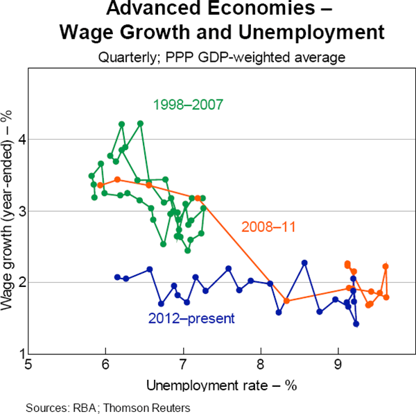
Since the global financial crisis (GFC), nominal wage growth has been sluggish across advanced economies. In aggregate, wage growth has remained low and little changed over the past 5 years while the unemployment rate has declined by around 3 percentage points (Graph 1).[1]
There are several possible explanations for this apparent disconnect between nominal wage growth and unemployment. Cyclical factors are likely to be important:
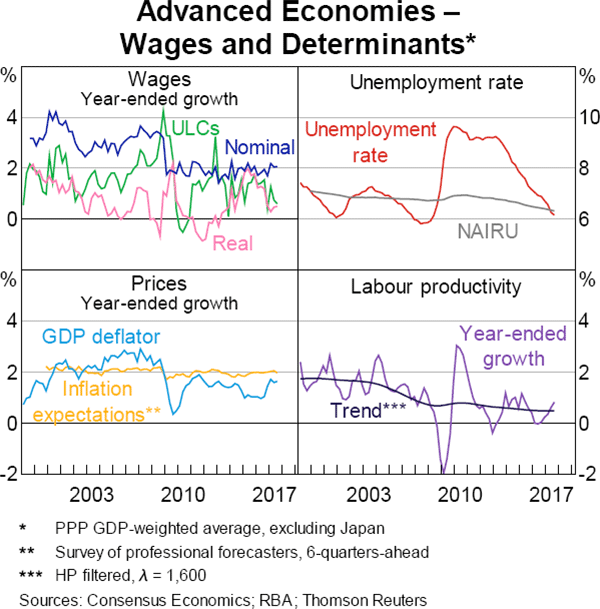
- It might take some time for wage growth to pick up, once unemployment has fallen to levels associated with ‘full employment’ (the non-accelerating inflation rate of unemployment or NAIRU). Given that these levels have been reached only recently in some advanced economies, there might be a lag before labour market tightness feeds into stronger wage growth (Graph 2). This lag might be longer than usual if firms' and workers' reluctance to cut wages had resulted in the level of wages being higher post-crisis than cyclical conditions warranted; wage growth would then remain subdued until this ‘overhang’ was worked off as the labour market tightened.
- Price inflation and inflation expectations have been lower than in the pre-crisis period. Measuring the true inflation expectations of workers and firms is difficult, but many measures of inflation expectations weakened significantly after 2010 (Adeney, Arsov and Evans 2017). Real wage growth has therefore been similar in the post-crisis period to the rates seen in the years leading up to the crisis.
- Recent research has also pointed to weak labour productivity growth as part of the explanation for low wage growth (Haldane 2017; Brouillette et al 2017); the lower labour productivity growth in part reflects cyclical weakness in investment after the GFC as well as lower total factor productivity growth (which is likely to be at least partly related to more structural factors). Nominal unit labour costs (ULC) growth, which measures wage growth relative to productivity growth, has been only a little lower than in the pre-crisis period.
Taking into account these factors suggests that, while nominal wage growth has clearly been lower, other wage growth measures – including real wages and unit labour costs – have been less subdued after the GFC.
In addition to these cyclical factors, structurally lower employee bargaining power may also be depressing wage growth. Bargaining power is difficult to measure and may, in part, be determined by the labour market conditions themselves. Common proxies suggest that bargaining power has shifted away from labour: unionisation rates have declined and labour markets have become more flexible across advanced economies. At the same time, automation, technological change, increasing global production integration and offshoring have affected some segments of the labour market (Danninger 2016; Jacobs and Rush 2015; OECD 2017). These changes may be perceived (rightly or wrongly) by workers as a reduction in job security and an increase in competitive pressures, and therefore could be contributing to supressing wage growth to some extent (Foster and Guttmann 2018).
How Important are Cyclical Factors?
One way to assess the importance of cyclical factors for explaining sluggish wage growth is to estimate Phillips curves for each advanced economy. Phillips curve models relate wage growth to a measure of spare capacity in the labour market, wage growth in the recent past, inflation, inflation expectations and productivity growth. In this article, spare capacity in the labour market is measured using a non-linear form of the unemployment gap (see Appendix A for details). This specification means that a one percentage point decrease in the unemployment rate has a larger effect on wages when the unemployment rate is already low. In addition, the model includes the change in the unemployment rate, which allows for the economic cycle to have an independent effect on wages from the unemployment gap. Inflation in this article is measured as the year-ended growth in the GDP deflator and inflation expectations are professional forecasters' expectations of year-ended consumer price inflation in six quarters time. The model also includes trend labour productivity growth as one of the drivers of wage growth.[2] The motivation for this is that in the long run, from a firm's perspective, an employee's real wage should track how much they can produce per unit of labour input (Abel, Burnham and Corder 2016).
There are multiple nominal wage measures available for most economies. Wages measures in the national accounts are broadly consistent across economies but are volatile and affected by compositional change. Country authorities often focus on ‘preferred’ wage measures which abstract from these issues, such as the Wage Price Index in Australia and the Employee Cost Index or the Average Hourly Earnings in the United States. This article presents results based on these preferred wage measures; though the results are broadly consistent using either the preferred or national accounts wage measures.[3]
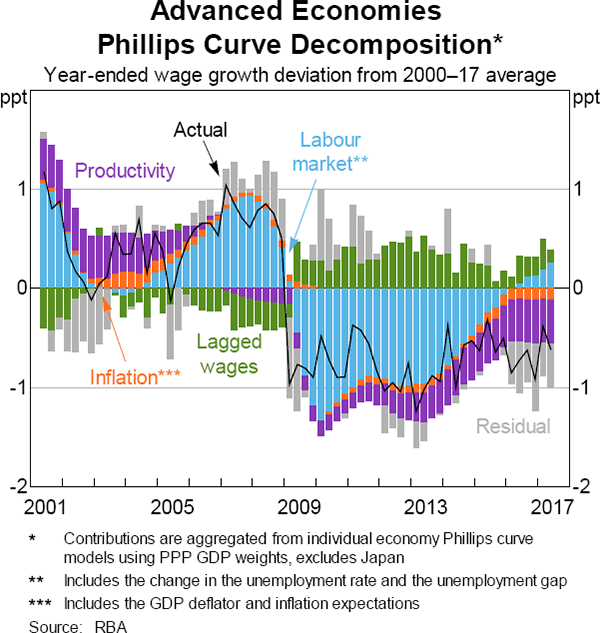
Overall wage developments over the past two decades are fairly well explained by these estimated Phillips curves, although over the past two years wages have been persistently weaker than estimated by the models (Graph 3). The fall in wage growth in 2009 is largely explained by the large amount of spare capacity that was created by the crisis. Most advanced economies experienced their deepest recessions since the Great Depression, and that was reflected in sharp increases in unemployment. Unemployment rates have been declining gradually since mid 2010, although that trend was interrupted in a number of economies by the euro area's sovereign debt crisis. The slow and protracted recovery has meant that labour market slack has placed downward pressure on wage growth for some time. However, labour market slack has been largely absorbed since mid 2016 and this should have pushed wage growth higher over the past one to two years.
Productivity growth has declined significantly since the mid 2000s; this also helps explain the slow growth in nominal wages over the past decade, and has been particularly relevant for wage growth in advanced economies since 2015. Subdued productivity growth accounts for much of the weakness in wage growth in the United States and New Zealand, and around a quarter of the weakness in the United Kingdom and Australia. A number of other recent studies have found a similar large role for productivity growth in explaining the sluggishness in wage growth in some economies (Pinheiro and Meifeng 2017). However, for the other advanced economies, labour productivity does not help to explain the low wage growth in recent years. The OECD (2017) reaches a similar conclusion, suggesting that low productivity growth is only part of the story.
The unexplained component of wage growth (measured by the residuals of the Phillips curve model) has become persistently and clearly negative; this pattern is evident across most of the economies in the sample. Since early 2016, wage growth in six of the nine advanced economies considered in this article has been consistently weaker than what is suggested by the Phillips curves for each of these economies.[4] Wage growth in Canada, the United Kingdom, Sweden, periphery euro area, the United States and Australia has been 0.4 and 1.2 percentage points lower on an average annualised basis than the estimated Phillips curve equations would suggest. This period of weaker-than-expected wage growth is not unprecedented – a similar pattern was observed in the early 2000s.
One explanation for the persistent negative residuals is that they are capturing measurement error. The recent combination of low unemployment and still low wage growth has prompted some questioning of whether unemployment is a sufficiently good measure of labour market spare capacity. There is only mixed evidence that other measures such as underemployment, measured by the share of the labour force that is in involuntary part-time employment, help to explain the weakness in wage growth in advanced economies (see Table 1 and discussion in the following section). In the case of Australia, Bishop and Cassidy (2017) suggest there is little empirical evidence that the level of underemployment has affected wage growth separately to unemployment. That said, other recent research has found that, at least for some advanced economies, the underemployment rate helps to explain the low wage growth (International Monetary Fund 2017). Alternatively, our measure of the unemployment gap might also be understating the amount of spare capacity in the labour market because estimates of the NAIRU are too high. The NAIRU is unobservable, changes over time and is estimated with a fair amount of uncertainty.
Has the Relationship between Labour Market Slack and Wage Growth Changed?
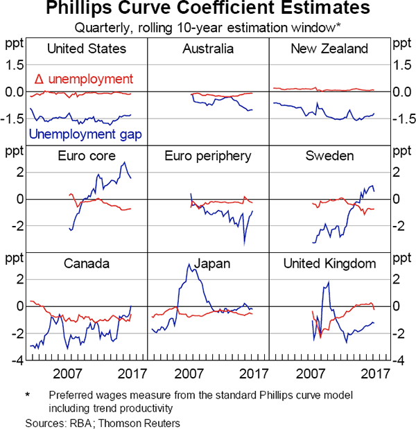
Another possible explanation for why wage growth has been weak is that wages may have become less responsive to changes in labour market slack after controlling for other variables in the Phillips curve. That is, the Phillips curve has flattened over time. Many reasons for such flattening have been proposed, including: increasing globalisation, particularly its potential effect on job security; declining bargaining power of workers from, for example, increasing automation; and legacy effects of the GFC. Estimating the Phillips curve equations over 10-year rolling windows can help uncover such flattening by examining how the coefficients on the unemployment gap and the change in the unemployment rate have evolved over time. A decline in the magnitude of these coefficients would suggest a flattening.
For the most part, the estimated coefficients for the unemployment gap and the unemployment rate have the expected signs. The estimates of the unemployment gap coefficient are negative and statistically significant most of the time (Graph 4). The relationship between wage growth and unemployment in the advanced economies outside of Europe does not appear to have substantially changed after the crisis. In the United States, both unemployment rate-related coefficient estimates have been remarkably stable since 2000. In Canada, the estimate of the gap coefficient is quite volatile, but the coefficient on the change in the unemployment rate has been fairly stable. In Australia and New Zealand, the estimates are fairly stable and, if anything, wage growth appears to have become more sensitive to the unemployment gap.
Overall, these results suggest that the link between wage growth and unemployment appears not to have been affected much by the GFC, at least according to this framework.[5] The main exceptions are some European Union economies. In the core euro area and Sweden, the coefficient on the unemployment gap has become positive since the GFC (though not statistically significant) and has increased over time. The ability for labour to move freely within the European Union may help explain this phenomenon, which points to a weaker relationship between wage growth and the local unemployment gap in the European Union economies that recovered more quickly from the crisis. In Japan, the gap coefficient has been zero over recent years; this reflects specific unique features of the Japanese labour market that are discussed further in Box A.
Box A Structural Factors and Wage Growth in Japan
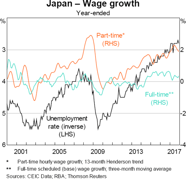
Japanese wage growth has remained subdued in recent years, despite Japanese labour market conditions appearing to be at their tightest in nearly three decades; the unemployment rate has declined to 20-year lows, the participation rate has increased noticeably, and the job vacancy rate has reached a multi-decade high. Much of the disconnect between wage growth and labour market conditions is due to Japanese-specific factors that are less relevant to other advanced economies. The main one of these is the high level of polarity in the Japanese labour market between ‘regular’ and ‘irregular’ employees. Regular employees participate in the traditional Japanese employment system with seniority-based remuneration and strong employee protections; these employees are almost invariably full time and have low job mobility (as at 2012, almost half of Japanese employees had job tenure of 10 years or over, compared to the OECD average of around 35 per cent). The economic stagnation in Japan since the early 1990s led to an increase in the share of irregular employees who have much weaker job protections, lower hourly wages and are often employed on a part-time basis. For example, the share of part-time workers has increased by around 5 percentage points over the past decade to almost one third of the labour force.
Full-time employees experience steady wage growth over their careers as their tenure increases, meaning that they are less likely to demand higher wage growth when labour market conditions are cyclically tight. Instead, they, and their labour unions, tend to focus on job security. Expectations of lifetime employment and strong employee protections for regular workers make it difficult for companies to adjust their labour input in economic downturns. Therefore, Japanese companies are less likely to hire full-time employees to meet fluctuations in demand or compete on wages for regular workers. As a result, full-time wage growth in Japan has been steady over the past two decades at around zero, even during periods when the unemployment rate had declined to very low levels such as in 2007–08 and, more recently, since 2013.
On the other hand, wages for part-time workers have been quite sensitive to the business cycle. Growth in hourly wages for part-time workers has increased steadily since 2012 as the labour market has tightened (Graph A1). One reason why wage growth for part-time workers has not yet surpassed the rate in 2009, when the unemployment troughed at a rate higher than it is currently, is that there has been a sizeable increase in Japanese labour force participation since 2012, implying that spare labour capacity existed beyond the unemployed. Much of that increase has been from females entering, or re-entering, the labour market, and many have been employed on a part-time/irregular basis.
Structural Factors and the Level of Wages
The persistent and unexplained weakness in wage growth over recent years points to the possibility that other factors have also contributed to wage growth developments (Graph 3). Many of these potential factors are structural in nature – such as a reduction in bargaining power or increasing globalisation.
Understanding their influences on wage growth presents several difficulties. Firstly, these factors cannot be observed directly and are difficult to measure. This can be addressed by using typical proxies for these variables: import penetration for globalisation; and the share of the labour force that is unionised together with a measure of employee protections to capture labour's bargaining power.[6] Secondly, the structural factors are slow moving, and the variables used to represent them are available only annually; as a result, they are measured at a lower frequency than the cyclical variables that have been typically thought to influence wage growth. This makes using the individual economy Phillips curve framework to understand the roles of these structural developments infeasible, due to the limited number of observations at the annual frequency.
Instead, a panel Phillips curve error correction model can be used to explore this question. This model relates wage growth to the long-run relationship between wages, productivity and prices; structural factors measuring changes in globalisation and labour's bargaining power; underemployment; and the cyclical variables included in the previous section. This approach assumes that each of the independent variables has the same effect on wage growth across the different economies (for more details on the model see Appendix C).[7] However, as is illustrated by the country-specific analysis of the role of the cyclical variables, this may not be the case. The Phillips curves estimates in the previous section show that the unemployment gap coefficients vary significantly across the advanced economies, which likely reflects differences in their labour market's flexibility and sensitivity to economic conditions. Alternative specifications, that are less restrictive in their assumption on the coefficients across economies, suggest that the results reported below broadly hold.[8]
Deviations in the level of wages from their long-run relationship with productivity and output prices are described by an error correction term.[9] In the core euro area economies and, to a lesser extent, in the periphery euro area economies, the error correction term was positive for a sustained period following the crisis. In other words, because of downward nominal wage rigidities and low inflation, it took a while for wages to adjust to weaker economic conditions. As a result, there was a period of downward pressure on wage growth until wages, prices and productivity were realigned (Graph 5). The United States, the United Kingdom and Canada had a similar wage overhang following the GFC, although wages in these economies adjusted more quickly, likely because of their more flexible labour markets. More recently, the level of wages in the United States, Canada and Australia also appeared to be elevated relative to productivity and output prices over the past two years. In Australia and Canada, this primarily reflected a sharp slowing in the GDP deflator, in part due to declines in commodity prices and the terms of trade.[10] In the United States, this largely reflected a further decline in labour productivity growth.
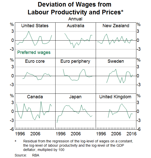
The results of the cross-country panel estimation suggest that both the level of wages and changes in labour's bargaining power help explain the pattern of wage growth across advanced economies (Table 1). Specifically, when wages in a given year are higher than what is implied by the estimated long-term relationship between wages, labour productivity and output prices, there is downward pressure on the subsequent year's wage growth. The implication is that wages tend to adjust slowly to changes in trend productivity growth and inflation, possibly because of nominal wage rigidities. Therefore, it appears that the sluggish wage growth in the aftermath of the GFC, in part, reflects a slow adjustment in nominal wages to cyclically weak economic conditions. This decline in the fundamental level of wages coincided with both lower productivity growth, with this slowdown starting a little before the GFC, and weak inflation caused by the severity of the recession. The analysis here suggests that a renewed wage overhang may help explain the weakness in nominal wages in 2017 in the United States, Canada and Australia.
| Coefficient | p-value | |
|---|---|---|
| Constant | 4.11 *** | (0.00) |
| Error correctiont −1/100 | −0.34 *** | (0.00) |
| ΔUnionisationt−1 | 0.27 *** | (0.01) |
| ΔEmployee protectionst−1 | 1.44 | (0.14) |
| Δlmport penetrationt−1 | 0.09 | (0.20) |
| Involuntary part timet | −0.24 *** | (0.00) |
| Unemployment gapt | −1.92 ** | (0.01) |
Inflation expectations |
−0.44 * | (0.09) |
ΔGDP deflator |
0.12 * | (0.06) |
| ΔUnemployment ratet | 0.26 ** | (0.04) |
| %ΔWagest−1 | 0.16 * | (0.06) |
|
(a) Unbalanced panel, not all economies have data from 1994; excludes Japan. Employee protections data are only available up to 2013. The panel is estimated up to 2016, with protections held constant for 2014 and 2015. This does not significantly change the coefficient estimates compared with estimating the panel up to 2014. Estimated with cross-section and year fixed effects. ***, **, * indicate significance at the 1, 5, and 10 per cent level, respectively. Source: RBA |
||
Structural changes in labour's bargaining power also help to reconcile some of the unexplained weakness in wage growth. Higher unionisation rates and stricter labour market protections are associated with stronger labour bargaining power. A more unionised labour force is likely to have a stronger negotiating position with employers and stricter labour market protections make the existing workers feel more secure in their jobs. Unionisation rates have declined across all advanced economies since at least the early 1990s (Graph 6). More recently, the decline in unionisation rates has been most pronounced in Australia, the euro area and New Zealand. The model estimates suggest that a decrease in the unionisation rate lowers wage growth in the following year; that is, it is associated with lower wages for a given level of labour market slack (and other model variables). Consistent with the union density results, lower employee protection also appears to lower wage growth the following year, though the effect is only marginally significant.[11]
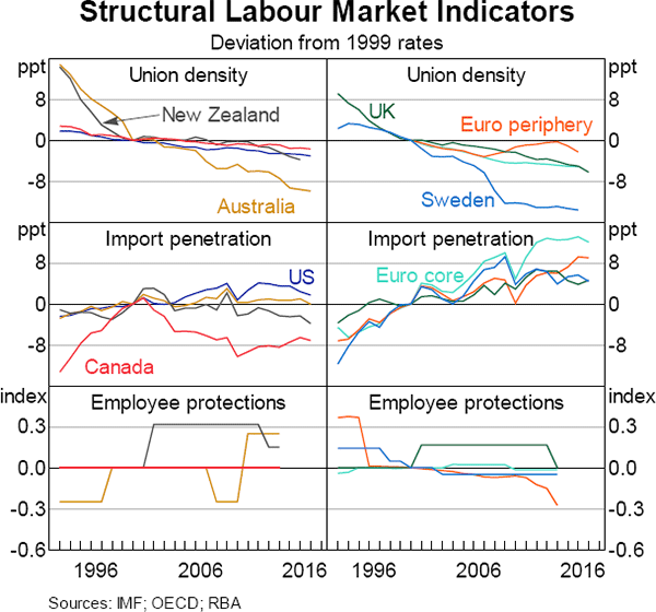
The coefficient on import penetration is positive (though not statistically significant across most specifications) which is inconsistent with the argument that increased competition from foreign workers has weighed on wage growth in the advanced economies. Potentially, the import penetration term may be capturing some offsetting productivity benefits of increased globalisation and supply chain integration above and beyond what is captured in the error correction term, given that stronger trade integration directly affects productivity growth and incentives to innovate (OECD 2017). Alternatively, the aggregate economy import penetration ratio may simply be too crude of a proxy for changes in workers' perceived job security resulting from increased competition. Foster and Guttmann (2018) find that in Australia, while import penetration ratios have increased across most industries, the effect of this on the aggregate labour market has been offset by stronger employment growth in industries that are less exposed to international trade.
Underemployment (measured as the share of the labour force that is in involuntary part-time work) appears to help explain developments in wage growth; the coefficient on the underemployment term is negative and statistically significant. However, this may be a consequence of the model assumptions, because, unlike the more robust results for the other variables, underemployment does not help explain the residuals from the Phillips curve equations presented in the previous section. The underemployment rate may be capturing similar information to the unemployment gap, which is unsurprising given that the two variables tend to move closely together in most economies. Indeed, the coefficient on the unemployment gap becomes much more economically significant when underemployment is excluded.
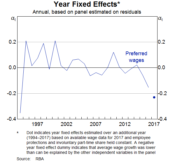
The cyclical variables that are thought to typically drive wage growth – labour market slack and inflation – augmented with productivity, measures of labour's bargaining power and globalisation still fail to fully explain the weakness in wage growth in advanced economies in recent years. This can be seen in the negative and statistically significant common residuals in 2016 and 2017 (Graph 7). It appears that some, as yet unidentified, common factor, or factors, have weighed on wage growth in recent years.
Conclusion
Nominal wage growth in advanced economies remains well below its pre-GFC average. Cyclical factors have played a significant part in this. Labour market slack has generally declined across advanced economies, but unemployment rates still remain above the rate consistent with full employment in a number of economies. A decline in labour productivity growth, which appears to have commenced a few years before the GFC, helps explain some of the recent wage weakness (especially in the United States). Wages growth might also have been weak recently because wages could adjust only slowly to the weak post-crisis economic conditions. Structural changes in the labour market, including declines in unionisation rates and employee protections also seem to be factors behind the weaker wage growth. However, all of these factors are only part of the story and, over the past two years, there appears to have been some other common factor weighing on wage growth across advanced economies.
Accommodative monetary policy, as well as other policies that can help stimulate demand, will further reduce labour market slack. This should support wage growth given that the cyclical relationship between labour market slack and wages does not appear to have changed dramatically in many economies. A cyclical recovery in investment in advanced economies would also contribute to capital deepening and a pick-up in labour productivity. To the extent that labour markets continue to tighten and investment continues to recover, these factors should contribute to further increases in wage growth.
Appendix A The Phillips Curve Model
The Phillips curve model for each advanced economy in the sample is based on Jacobs and Rush (2015) but is augmented with trend labour productivity growth:
Where:
- wt is quarterly growth in the seasonally adjusted nominal wage
-
 is the unemployment gap which is non-linear in the unemployment rate (ut)
(as specified in Debelle and Vickery 1997).
  is the NAIRU. NAIRUs
are the latest estimates available from the relevant sources for each economy:
Reserve Bank of Australia (Australia), Congressional Budget Office (United
States), European Commission (euro area economies and Sweden), OECD (all
other economies). The estimation methods of the different sources are broadly
based on inferring the NAIRU from a Phillips curve type relationship, the
details and methodologies may vary and influence the estimates
- Δut is the change in the unemployment rate
-
 is year-ended growth rate in the GDP deflator
-
 is year-ended inflation expectations in 6 quarters time from surveys of professional
forecasters. The choice of these particular inflation expectations reflects
their availability across the advanced economies.
- Δzt is quarterly growth in trend labour productivity (measured as output per employee and as reported by the OECD; trend productivity places less weight on quarterly variation which could be influenced by measurement error in labour inputs). Trend productivity is calculated using a Hodrick-Prescott filter with a smoothing parameter of 1,600. This particular measure has well-known end point issues but alternative measures produce similar results.
Equation A1 is estimated using ordinary least squares with heteroscedasticity-consistent standard errors on quarterly data. This approach assumes a standard and common Phillips curve specification across all economies. It only allows for cross-country differences in the wage data generation process via the coefficient estimates (which are specific to each economy), rather than model specification.
Appendix B Wage measures
| Wage measure | Definitional notes | Source | Estimation period (preferred wages) | Estimation period (OECD wages)(a) | |
|---|---|---|---|---|---|
| Australia | Wage Price Index | Per hour; adjusts for changes in labour quality and compositional effects; excludes bonuses. | ABS | 1998–2017 | 1991–2017 |
| Canada | Compensation per hour | Business sector | Statistics Canada | 1993–2017 | 1993–2017 |
| Core euro area | Compensation per employee | Gross wages and salaries, as well as bonuses, overtime payments and employers' social security contributions | ECB | 1997–2017 | 1997–2017 |
| Periphery euro area | Compensation per employee | Gross wages and salaries, as well as bonuses, overtime payments and employers' social security contributions | ECB | 1998–2017 | 1998–2017 |
| Japan | Nominal Wage Index | Average total wages, all employees | Statistics Bureau / RBA | 1995–2017 | 1995–2017 |
| New Zealand | Labour Cost Index | Includes base salary rates, ordinary time wage rates, and overtime wage rates | Statistics New Zealand | 1995–2017 | 1995–2017 |
| Sweden | Labour cost for LCI | Employee compensation, wages and salaries in cash and in kind, social security contributions and employment taxes regarded as labour costs minus subsidies received, per hour | Eurostat | 1999–2017 | 1995–2017 |
| United Kingdom | Average weekly earnings | Includes bonuses | ONS | 2000–2017 | 1990–2017 |
| United States | Average of Employment Cost Index (ECI); compensation per hour; median weekly earnings; and average hourly earnings | Simple average of four wages measures; ECI adjusts for compositional changes; compensation per hour is for the non-farm business sector; average hourly earnings is for non-farm production and non-supervisory employees | BLS / RBA | 1993–2017 | 1993–2017 |
|
(a) The OECD measure is based on a national accounts measure of wages per employee (wage rate, total economy) |
|||||
Appendix C The Panel Model
The dependent variable in the annual panel model used in this article is annual wage growth. The panel is estimated with cross-section and year fixed effects:
Where subscript i represents each country, subscript t represents each time period and Xj,i,t is a vector of the annual averages of the j cyclical variables (excluding labour productivity) included in equation A1. As a robustness check, a version of the model is also estimated with the annual average of the residuals from equation A1 as the dependent variable (columns I, III and IV in Table C1), and without the vector of cyclical variables (Xj,i,t). In this case the model is estimated using year fixed effects. In general, results are consistent across these two specifications for each wage measure, though there are some differences in the results between wages measures. For example, unionisation rates appear to be more important when using the preferred wages measure, while employee protections appear to be more important for the national accounts wages measure. In general, the importance of the level of wages (based on the error correction term) and bargaining power (whether defined by unionisation rates or employee protections) appear to be important across all specifications.
In regressions I, II, III and V the error correction term (specifically, ∈t from the equation ln Wagest = γ1 + γ2 ln Labour Productivityt + γ3 ln GDPdeft + ∈t) is estimated without coefficient restrictions. This allows for trends in the labour share of income over the estimation period, which is consistent with the data for most economies. As a robustness check, Equation IV is estimated with an error correction term with coefficient restrictions on the long run relationship between national accounts wages, prices and productivity (γ2 = γ3 = 1). The validity of the constrained approach assumes that the labour share of income is fairly stable over the estimation period.
| Preferred wages measure | National account wages measure | |||||||||
|---|---|---|---|---|---|---|---|---|---|---|
| Residual(b) | Wage growth(c) | Residual(b) | Residual(d) | Wage growth(c) | ||||||
| I | II | III | IV | V | ||||||
| Coef | p-value | Coef | p-value | Coef | p-value | Coef | p-value | Coef | p-value | |
| Constant | 0.03 | (0.47) | 4.11 | (0.00) | 0.00 | (0.98) | 0.00 | (0.94) | 2.34 | (0.01) |
| Error correctiont−1/100 | −0.04 | (0.01) | −0.34 | (0.00) | −0.06 | (0.00) | −0.01 | (0.30) | −0.37 | (0.00) |
| ΔUnionisationt−1 | 0.04 | (0.07) | 0.27 | (0.01) | 0.05 | (0.16) | 0.05 | (0.15) | 0.24 | (0.05) |
| ΔEmployee protectionst−1 | 0.19 | (0.50) | 1.44 | (1.14) | 0.75 | (0.05) | 0.80 | (0.05) | 2.90 | (0.02) |
| Δlmport penetrationt−1 | 0.02 | (0.24) | 0.09 | (0.20) | 0.06 | (0.02) | 0.04 | (0.08) | 0.19 | (0.02) |
| Involuntary part timet | 0.00 | (0.76) | −0.24 | (0.00) | 0.00 | (0.92) | 0.00 | (0.78) | −0.12 | (0.17) |
| Unemployment gapt | -- | -- | −1.92 | (0.01) | -- | -- | -- | -- | −2.27 | (0.00) |
Inflation expectations |
-- | -- | −0.44 | (0.09) | -- | -- | -- | -- | 0.14 | (0.54) |
ΔGDP deflator
|
-- | -- | 0.12 | (0.06) | -- | -- | -- | -- | 0.19 | (0.02) |
| ΔUnemployment ratet | -- | -- | 0.26 | (0.04) | -- | -- | -- | -- | 0.02 | (0.90) |
| %ΔWagest−1 | -- | -- | 0.16 | (0.06) | -- | -- | -- | -- | 0.22 | (0.00) |
|
(a) Unbalanced panel, not all economies have data from 1994; excludes
Japan. Employee protections data are only available up to 2013. The
panel is estimated up to 2016, with protections held constant for 2014
and 2015. This does not significantly change the coefficient estimates
compared with estimating the panel up to 2014. Source: RBA |
||||||||||
Footnotes
The authors are from Economic Analysis Department, and thank Meika Ball (also from the Economic Analysis Department) for her contribution on the Japanese labour market in Box A. [*]
The advanced economies covered in the article are Australia, Canada, Japan, New Zealand, Sweden, the United Kingdom and the United States, as well as aggregates for the ‘core euro area’ (Austria, France, Germany and the Netherlands) and the ‘periphery euro area’ (Ireland, Italy, Portugal and Spain). The euro area aggregates are used to reflect the different developments within the euro area, with the periphery more heavily impacted by the GFC and the subsequent euro area debt sovereign crisis. [1]
The usual Phillips curve specification does not include productivity growth as a driver of nominal wage growth. However, recently there has been a heightened focus on the role of productivity because of its prolonged weakness after the GFC. To address its potential role across the advanced economies the Phillips curve specification used in the article includes productivity growth. Productivity measures tend to be noisy. Trend productivity places less weight on quarterly variation which could be influenced by measurement error. This article measures trend productivity with a Hodrick-Prescott filter with a smoothing parameter of 1,600. Different trend measures tend to produce similar results as reported here (International Monetary Fund 2017). [2]
For more details on the wage measures used for each economy see Appendix B. [3]
Based on Phillips curves estimated from the mid 1990s to 2017. See Table B1 for the full-sample estimation period. [4]
The BIS (2017) also reaches a similar conclusion for the G7 economies over a somewhat longer period starting in the early 1990s. [5]
Import penetration is the share of domestic demand (GDP less net exports) which is met by imports: Import penetration = 100 × imports/(GDP − exports + imports). Import penetration is one common way to measure globalisation (OECD 2010). Employee protections are based on an OECD-constructed measure. [6]
By construction, a panel estimates one coefficient for each variable across each of the cross-sections. Trends in wage growth in Japan are partly the result of structural features specific to the Japanese labour market. As such, Japan is excluded from the panel estimation. See Box A for more information. [7]
To check that these restrictions are not influencing the results, the panel is also estimated on the annual average unexplained wage component (i.e. the residuals from equation A1), rather than on annual wage growth directly. This allows for differences in the relative effects of the cyclical variables across advanced economies; the results (reported in Table C1) and conclusions are broadly similar. [8]
Specifically this term is the residual ∈t from the regression of the log level of wages on the log level of productivity (actual, not trend) and output prices: ln Wagest = γ1 + γ2 ln Labour Productivityt + γ3 ln GDPdeft + ∈t. [9]
Changes in the GDP deflator due to commodity prices may not be a good description of the aggregate pricing environment faced by firms weighted by their share of employment. The mining sector is comparatively more capital intensive and requires less labour input per unit of output. [10]
The effect of employee protection is statistically significant for the national accounts measure of wages. Employee protections data are based on the OECD Indicators of Employment Protection. Employment protections strictness based on: protection of regular workers against individual dismissal; regulation of temporary forms of employment; and additional, specific requirements for collective dismissals. [11]
References
Abel W, R Burnham and M Corder (2016), ‘Wages, productivity and the changing composition of the UK workforce’, Bank of England Quarterly Bulletin 2016 Q1.
Adeney R, I Arsov and R Evans (2017), ‘Inflation Expectations in Advanced Economies’, RBA Bulletin, March, pp 31–44.
Bank for International Settlements (2017), ‘87th Annual Report, 2016/17’, 25 June. Available at <http://www.bis.org/publ/arpdf/ar2017e.htm>.
Bishop J and N Cassidy (2017), ‘Insights into Low Wage Growth in Australia’, RBA Bulletin, March, pp 13–20.
Brouillette D, J Ketcheson, O Kostyshyna and J Lachaine (2017), ‘Wage Growth in Canada and the United States: Factors Behind Recent Weakness’, Bank of Canada Staff Analytical Note 2017–8.
Danninger S (2016), ‘What's Up with U.S. Wage Growth and Job Mobility?’, IMF Working Paper WP/16/122.
Debelle G and J Vickery (1997), ‘Is the Phillips Curve A Curve? Some Evidence and Implications for Australia’, Research Discussion Paper 9706, October.
Foster J and R Guttmann (2018), ‘Perceptions of Job Security in Australia’, RBA Bulletin, March.
Haldane AG (2017), ‘Work, wages and Monetary Policy’, Speech at the National Science and Media Museum, Bradford, 20 June. Available at <http://www.bankofengland.co.uk/publications/Documents/speeches/2017/speech984.pdf>.
International Monetary Fund (2017), ‘Recent Wage Dynamics in Advanced Economics: Drivers and Implications’, World Economic Outlook, October, pp 73–116.
Jacobs D and A Rush (2015), ‘Why Is Wage Growth So Low?’, RBA Bulletin, June, pp 9–18.
OECD (2010), Measuring Globalisation: OECD Economic Globalisation Indicators 2010, OECD Publishing, Paris.
OECD (2017), ‘General Assessment of the Macroeconomic Situation’, OECD Economic Outlook, 2017 Issue 1, pp 11–60.
Pinheiro R and Y Meifeng (2017), ‘Wage Growth after the Great Recession’, FRB Cleveland Economic Commentary 2017-04.

