Bulletin – June 2017 Australian Economy Estimating the NAIRU and the Unemployment Gap

What Is the NAIRU and Why Is It Important?

Labour underutilisation is an important consideration for monetary policy. Spare capacity in the labour market affects wage growth and thus inflation (Graph 1). Reducing it is also an end in itself, given the Bank's legislated mandate to pursue full employment. The NAIRU – or non-accelerating inflation rate of unemployment – is a benchmark for assessing the degree of spare capacity and inflationary pressures in the labour market. When the observed unemployment rate is below the NAIRU, conditions in the labour market are tight and there will be upward pressure on wage growth and inflation. When the observed unemployment rate is above the NAIRU, there is spare capacity in the labour market and downward pressure on wage growth and inflation. The difference between the unemployment rate and the NAIRU – or the ‘unemployment gap’ – is therefore an important input into the forecasts for wage growth and inflation.

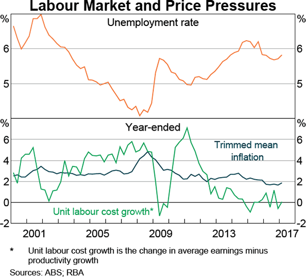
In practice, the NAIRU – and therefore the unemployment gap – are not observed. This article sets out how the Bank currently estimates the NAIRU for the purpose of forecasting wage growth and inflation, and how estimates of the NAIRU have changed over time.^[1]

The NAIRU can be defined in various ways and is sometimes used interchangeably with the broader concept of the unemployment rate associated with ‘full employment’. In this article we use a narrower definition and define the NAIRU as the unemployment rate that is consistent with inflation converging to the rate of long-term inflation expectations in the economy. This approach has proven useful for modelling inflation. Other approaches to estimating the NAIRU (or full employment) are intuitively appealing but less useful for modelling inflation. For example, the NAIRU can be modelled as a function of observable variables like labour market regulation (e.g. minimum wages), union membership rates, the level of unemployment benefits, and demographics. Another approach defines full employment using types of unemployment, which can be linked to observable characteristics. Full employment occurs when there is no cyclical unemployment, and the only unemployment is either structural or frictional (e.g. Ballantyne et al 2014). Models can include labour market dynamics such as longer durations of unemployment leading to skills atrophy and decreased employability (e.g. Ball 2009). Some researchers connect the NAIRU to the rates at which employees find and leave jobs (e.g. Dickens 2009). These other methods can be used for exploring the economics of why the NAIRU might change. However, the method in this article aims only to detect changes in the NAIRU, not explain them.

Estimating the NAIRU

The NAIRU is not observable, but we can infer it from the relationship between the unemployment rate and inflation (or wage growth). In this article, the NAIRU is the unemployment rate at which inflation converges to the level of long-run inflation expectations. If the NAIRU was constant over time, it could be estimated using a simple regression of inflation against the unemployment rate.^[2] However, evidence suggests that the NAIRU changes over time and models that allow the NAIRU to vary generally have greater predictive power for inflation and wage growth (e.g. Gruen et al 1999; Ball and Mankiw 2002).

To estimate a NAIRU that varies over time requires a more complex model. Inflation and wage growth are affected by the unemployment gap (among other things). The gap cannot be observed directly, but the relationship between the unemployment gap and inflation means we are able to infer changes in the gap by observing inflation outcomes, controlling for other things. More concretely, if inflation is lower than expected, a possible explanation is that the unemployment gap was larger than we thought. In response, we might lower our estimate of the NAIRU. We use a statistical technique known as the Kalman filter to calculate how much we should revise our estimate of the NAIRU based on new data. For example, our model suggests we should increase our estimate of the NAIRU by just over ¼ of a percentage point in response to quarterly inflation being ½ percentage point higher than expected in that quarter.

The unemployment gap also affects wage growth. Conceptually, the NAIRU should be the same whether we use inflation or wage growth to estimate it. However, in practice, the estimate varies if you use inflation or use wage growth (e.g. Gruen et al 1999 and Ballantyne et al 2014). The method used here derives a single estimate of the NAIRU using information from both inflation and wage growth.

The model

The model comprises separate equations for inflation, wage growth and the NAIRU. Inflation and wage growth are modelled using lags of themselves and each other, long-term inflation expectations, the unemployment gap, the change in the unemployment rate, and import prices (more details in Appendix A). Oil prices appear in both equations, but only prior to 1977 when they were correlated with large changes in prices and wages.^[3] Inflation is measured by quarterly trimmed mean inflation. Wage growth is measured by growth in unit labour costs (ULCs), defined as average earnings growth adjusted for productivity growth. Strictly speaking, the ULC measure used here includes more than just wages. By incorporating productivity as well, it becomes more relevant for inflation forecasting. The model also includes an equation for the evolution of the unobservable NAIRU. We do not model the structural determinants of the NAIRU. The baseline assumption is that it will stay constant in the next period.

The NAIRU estimates

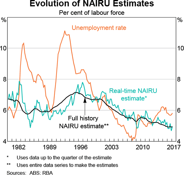
Central estimates of the NAIRU from the model, as well as the uncertainty around these estimates, are presented in Graph 2. The estimated NAIRU peaked in 1995 at just over 7 per cent of the labour force and has declined more or less steadily since then to around 5 per cent in early 2017. While the structural determinants of the NAIRU are not modelled here, other research has attempted to explain changes in the NAIRU. The results of that research are far from conclusive, but OECD studies provide some possible explanations.^[4] Those studies suggest that the increase in unemployment benefits as a share of average wages from the mid 1970s to the early 1990s, and their subsequent decline, influenced the rise and fall in the NAIRU. Decreases in trade union membership and product market regulation are also estimated to have lowered the NAIRU since the mid 1990s. The studies did not find any evidence that the level of the minimum wage affected the NAIRU.

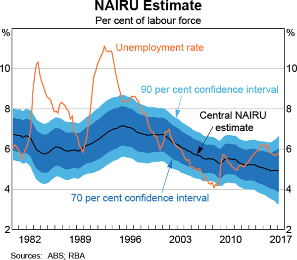
Economic conditions may also have delayed effects on the NAIRU. Long periods of unemployment can decrease an individual's future employment opportunities, perhaps because of real or perceived skills attrition. These long periods out of work tend to occur more often when the unemployment rate is high. This process – known as hysteresis – can raise structural unemployment and often follows rapid increases in the unemployment rate during recessions. When the labour market is tight, employers are more likely to hire workers with less desirable work histories or characteristics. A period of employment often improves a person's future job prospects, which may lower structural unemployment. In Australia, the rise in the estimated NAIRU between 1984 and 1995 occurred alongside two recessions. Conversely, the fall in the NAIRU over the past 20 years has occurred during a prolonged period of economic growth.

We can use the central estimates of the NAIRU to construct estimates of the unemployment gap. The relatively smooth evolution of the estimated NAIRU through time suggests that most of the short-term variation in the unemployment gap comes from observable changes in the unemployment rate.^[5] It also suggests that movements in the NAIRU have been driven by slow-moving structural features of the labour market, which are typically hard to observe.

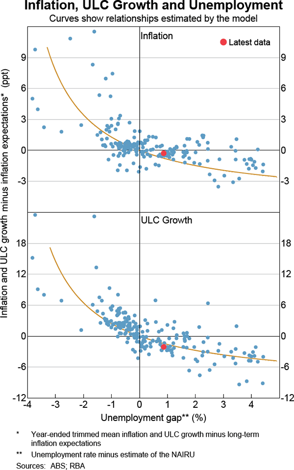
The relationship between the estimated unemployment gap and inflation, relative to long-run expectations, is shown in Graph 3. As expected, inflation tends to be higher when the unemployment gap is negative (i.e. when the observed unemployment rate is below the NAIRU). Similarly, wage growth tends to be higher when the unemployment gap is negative. Both relationships are nonlinear, so increases in the unemployment gap have less of an effect on inflation and wage growth as the unemployment gap increases. If there are already many unemployed workers looking for a job, a few more are unlikely to have much effect on the wage offered.

NAIRU estimates are uncertain, especially in real time

Estimates of the NAIRU are uncertain because it cannot be observed and the data provide only a noisy signal. The current estimate of the NAIRU is 5.0 per cent of the labour force, with a 70 per cent confidence interval of plus or minus 1 percentage point. This means that, even if the models of inflation and wage growth are right, there is still a 30 per cent chance that the ‘true’ unobserved NAIRU is either higher than 6 per cent or lower than 4 per cent (Graph 2). Given the March quarter unemployment rate of 5¾ per cent, the model suggests an 80 per cent chance that the unemployment rate is above the NAIRU.

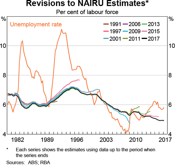
The central estimates of the NAIRU presented in Graph 2 use the full history of the data. However, the path of the NAIRU estimated now can look quite different to the path estimated at various times in the past, even using the same model and data history. The high degree of uncertainty around the NAIRU estimates means new data can change the estimate of the NAIRU for the previous few years. Graph 4 shows how the revisions to the NAIRU estimate have unfolded over time.^[6] Each series shows the NAIRU estimate based on the data up to that time period. For example, the estimates made using data up to the December quarter of 2015 showed the NAIRU had been fairly flat over the previous two years and was around 5.2 per cent. But by the March quarter of 2017, the latest estimates show the NAIRU had been falling over that same period and was 5.0 per cent in the March quarter of 2015.

When updating the economic forecasts each quarter, Bank staff use the latest estimate of the NAIRU as an input into the forecasts for inflation and wage growth. Because of the uncertainty around the NAIRU, the estimates generated by incorporating new data each quarter can move around much more sharply than the estimates made with the benefit of hindsight and the full history of the data. Graph 5 shows estimates of the NAIRU through time that use only the data available up to that time period, compared with estimates that use the full data history. The real-time series shows the estimate of the NAIRU the model would have made for each quarter at that time. These real-time estimates give a better sense of the uncertainty faced by forecasters than the estimates using the full history.^[7]

Inflation expectations and the NAIRU

In the model, the unemployment gap drives deviations of inflation and wage growth from long-term inflation expectations. This means that estimated movements in the NAIRU depend on which measure of inflation expectations is used. Previous versions of the model used inflation expectations derived from 10-year bond rates. Moore (2016) examines a wide range of measures of inflation expectations available in Australia. Expectations measures derived from bond rates do not purely reflect inflation expectations because they also include risk and liquidity premia. Each measure has pros and cons, so in this model we combine a range of measures of inflation expectations (Graph 6). Specifically, we extract a common signal of long-term expectations from the various measures after controlling for each measure's co-movement with recent inflation.^[8]

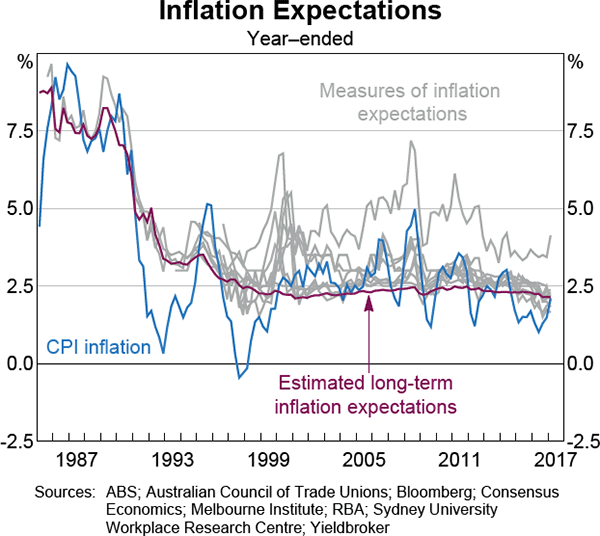
The average level of the inflation expectations measure used in the model also affects the level of the NAIRU estimates. Many of the measures of inflation expectations appear to be upwardly biased (as tends to be the case for other economies), which would result in a downward bias in the NAIRU estimate. To avoid this problem, we adjust the mean of the estimated inflation expectations series to match the mean of inflation since 1996, which is roughly the period when expectations appear to have been anchored around the inflation target.

The NAIRU and Recent Weakness in Wage Growth

Our model of inflation and wage growth accounts for the effects of a number of observable variables. However, there are other variables that can affect inflation and wage growth that are not included in the model (for example, because of insufficient data). If these omitted variables change and cause inflation or wage growth to deviate from the model predictions, some of this deviation will be attributed to changes in the NAIRU. Therefore the model's estimate of the NAIRU could change, even though the ‘true’ unobservable NAIRU might not have.

Recent RBA work has considered some possible explanations for low wage growth that do not correspond to variables in the model.^[9] Decreased bargaining power of labour and relatively high underemployment are two of the explanations canvassed. We look at how these explanations could affect model estimates of the NAIRU.

Decreased employee bargaining power

If employees have less bargaining power, then one would expect to see lower wage growth (all else equal). Because bargaining power is not in the model, wage growth would be lower than predicted and the NAIRU estimate would fall. If a reduction in bargaining power is sustained, the NAIRU estimate would continue to fall. A permanent decrease in bargaining power would lead the NAIRU to decline to a lower level reflecting decreased wage pressures at any given unemployment rate. However, if bargaining power were to increase after a temporary reduction, wage growth would start surprising the model on the upside and the estimate of the NAIRU would increase again.

Bargaining power is not an observable variable. This means that the model cannot tell us whether any given change in the NAIRU is caused by a change in bargaining power. The model deals with this by treating all unmodelled changes in wage growth the same way. It estimates how much of each change is temporary versus how much is permanent, based on historical experience.

Relatively more underemployment

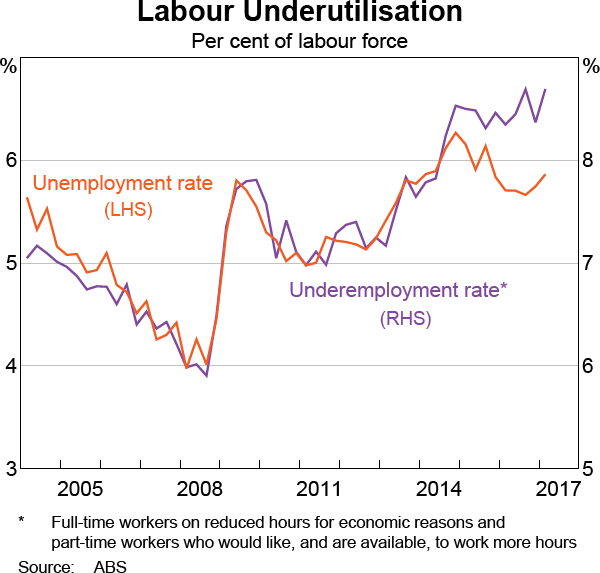
The underemployment rate measures the number of employed people who would like, and are available, to work additional hours, expressed as a share of the labour force (Graph 7).

The model in this article does not include the underemployment rate, but it does include the unemployment rate.^[10]

Between 2004 and 2014, the underemployment rate tended to move fairly closely with the unemployment rate. This meant the unemployment rate was a reasonable proxy for any effect that changes in the underemployment rate had on wage growth. Over the past few years, however, the underemployment rate has been relatively stable while the unemployment rate has declined. Any effect of the underemployment rate on wage growth – over and above the effect of the unemployment rate – would result in lower wage growth than expected by the model. This would then cause the model's estimate of the NAIRU to decline. This explanation implies that the unemployment gap, as measured using the unemployment rate, is currently understating the degree of spare capacity in the labour market. The model estimate of the NAIRU is then revised down to get a larger unemployment gap.

Conclusion

Estimates of the NAIRU are an input into the Bank's inflation and wage forecasts, which in turn feed into monetary policy decisions. The model-based estimates of the NAIRU presented in this article do not rely directly on structural features of the labour market, but are inferred from departures from the expected relationship between unemployment and inflation or wage growth. There is substantial uncertainty around these estimates of the NAIRU, especially in real time. This uncertainty means that the model's estimate of the NAIRU can change quite a bit from quarter to quarter as new data become available, even though we think the ‘true’ unobserved NAIRU actually evolves quite slowly.

Appendix A: Estimating the Model

The model comprises equations for inflation and wage growth as well as for the NAIRU. Details of the variables used are in Table A1.

View MathML

View MathML

View MathML

We estimate the model by maximum likelihood using the Kalman filter. Given the parameters, and an initial value for the NAIRU in 1968, the Kalman filter generates estimates of the NAIRU based on the data available up to each time period. The NAIRU is then projected forward one period (as per Equation (A3)). Along with the observable variables, this generates a prediction for inflation and wage growth for the period ahead (as per Equations (A1) and (A2)). Any difference between the prediction and the actual data will cause some revision to the NAIRU estimate for that quarter. The process is then repeated for the next quarter.

Stepping through the quarters gives a series of prediction errors, which depend on the parameter values. The maximum likelihood estimation routine finds the parameters that minimise those errors and give the best fit to the inflation and wage growth data. The results of estimation are in Table A2.

A statistical smoothing method is then used to construct the estimates based on the full history of the data. The smoothing method steps backward in time from the current period, updating the real-time NAIRU estimates in light of more recent data.

Table A1: Variable Descriptions and Data Sources

Variable	Description	Source
Δpt	Quarterly trimmed mean inflation; prior to 1978 it is weighted median inflation	ABS
	Long-term inflation expectations (on a quarterly basis)	Separate model estimates
Δulct	Quarterly unit labour costs growth, defined as growth of average earnings less productivity growth	Constructed from ABS data
Ut	Unemployment rate	ABS
	Year-ended growth in the consumer imports price deflator	ABS
Δoilt	Quarterly log change in Brent oil price (multiplied by 100)	Thomson Reuters
NAIRUt	Current estimate of the non-accelerating inflation rate of unemployment
D76	A dummy variable that is one prior to 1977
	The error in the inflation equation
	The error in the ULC equation
	The error in the NAIRU equation
Source: RBA

Table A2: Parameter Estimates

Estimation sample is March 1968 to March 2017

	Inflation equation		ULC growth equation
	Coefficient(a)	Standard error	Coefficient(a)	Standard error
	0.35***	0.06	0.45**	0.22
Δpt−1	0.24***	0.06	0.47**	0.22
Δpt−2	0.16***	0.05	0.09	0 .16
Δpt−3	0.18***	0.06
Δulct−1	0.06***	0.02
	−0.70	0.53	−5.6***	1. 7
	−0.38***	0 .10	−1.9***	0.53
	0.004	0.006
Δoilt−2(b)	0.02***	0.01	0.05***	0.01
σmeasurement(c)	0.30***	0.02	1.17***	0.06
	NAIRU equation
	Coefficient(a)		Standard error
σNAIRU(c)	0.40***		0.13
(a) *, ** and *** denote P values less than 0.1, 0.05 and 0.01 respectively (b) Prior to 1977 only (c) Standard deviation estimates, the errors are assumed to be distributed normally with mean zero and variance σ2 Source: RBA

Footnotes

The author is from Economic Analysis Department. [*]

The current estimation method builds on earlier work. See Gruen, Pagan and Thompson (1999) and Ballantyne, De Voss and Jacobs (2014) for details. [1]

In this case, the estimate of the constant NAIRU since 1966 would be 4½ per cent. This is found by estimating the NAIRU as a parameter in the inflation and wage equations in Appendix A, and then averaging them together. [2]

The strong correlation between oil prices and inflation and wage growth seemed to break down after the first oil shock. This may have been due to changes in institutional arrangements or a decreased share of oil in production, but our motivation is mostly empirical so the precise explanation is not important here. Oil prices do affect headline inflation, but that is not modelled here. [3]

See Bassanini and Duval (2006) and Gianella et al (2008) for details. [4]

The variability of the NAIRU is estimated from the data, rather than being assumed by the statistical procedure. [5]

Graph 4 shows a selection of estimates of through time. View an animated version of this graph showing the full history of estimates. [6]

A further source of real-time uncertainty is that new data can cause revisions to parameter estimates. Each new data point allows the parameters as well as the NAIRU to be re-estimated. However, over the past two decades the contribution of parameter re-estimation to real-time uncertainty has been very small. [7]

See Kozicki and Tinsley (2012) and Chan, Clark and Koop (2015) for details of similar estimates made on US data. [8]

See Lowe (2016), Davis, McCarthy and Bridges (2016) and Bishop and Cassidy (2017). [9]

Inflation models do not typically include the underemployment rate, in part because it tends to be correlated with the unemployment rate. Further research is looking into separately identifying the effects of underemployment. [10]

References

Ball L (2009), ‘Hysteresis in Unemployment: Old and New Evidence’, NBER Working Paper No 14818.

Ball L and G Mankiw (2002), ‘The NAIRU in Theory and Practice’, Journal of Economic Perspectives, 16(4), pp 115–136.

Ballantyne A, D De Voss and D Jacobs (2014), ‘Unemployment and Spare Capacity in the Labour Market’, RBA Bulletin, September, pp 7–20.

Bassanini A and R Duval (2006), ‘Employment Patterns in OECD Countries: Reassessing the Role of Policies and Institutions’, OECD Social, Employment and Migration Working Papers No 35.

Bishop J and N Cassidy (2017), ‘Insights into Low Wage Growth in Australia’, RBA Bulletin, March pp 13–20.

Chan J, T Clark and G Koop (2015), ‘A New Model of Inflation, Trend Inflation, and Long-Run Inflation Expectations’, Federal Reserve Bank of Cleveland Working Paper No 15–20.

Davis K, M McCarthy and J Bridges (2016), ‘The Labour Market during and after the Terms of Trade Boom’, RBA Bulletin, March, pp 1–10.

Dickens W (2009), ‘Has the Recession Increased the NAIRU?’, Brookings Report.

Gianella C, I Koske, E Rusticelli and O Chatal (2008), ‘What Drives the NAIRU? Evidence from a Panel of OECD Countries’, OECD Economics Department Working Papers No 649.

Gruen D, A Pagan and C Thompson (1999), ‘The Phillips Curve in Australia’, RBA Research Discussion Paper 1999-01.

Kozicki S and P Tinsley (2012), ‘Effective Use of Survey Information in Estimating the Evolution of Expected Inflation’, Journal of Money, Credit and Banking, 44(1), pp 145–169.

Lowe P (2016), ‘Inflation and Monetary Policy’, Address to Citi's 8th Annual Australian & New Zealand Investment Conference, Sydney, 18 October.

Moore A (2016), ‘Measures of Inflation Expectations in Australia’, RBA Bulletin, December, pp 23–31.