Bulletin – December 2016 Australian Economy The Sensitivity of Personal Income to GDP Growth
- Download 417KB
Abstract
This article examines how the income of different individuals varies in response to changes in the state of the economy using individual-level data from the Household, Income and Labour Dynamics in Australia (HILDA) Survey. More specifically, the article explores which types of income earners (those in the top, middle or bottom of the income distribution) and which sources of income (labour or capital) are most affected by economic conditions. Results suggest that the incomes of bottom- and top-income earners are the most sensitive to the state of the economy, although for different reasons: during strong economic conditions, the labour income of bottom-income earners rises, due to lower unemployment, while the capital income of top-income earners also rises, due to higher dividend and interest earnings. The effect on bottom-income earners appears to be stronger than that on top-income earners, suggesting that income inequality declines when economic conditions are strong.
Introduction
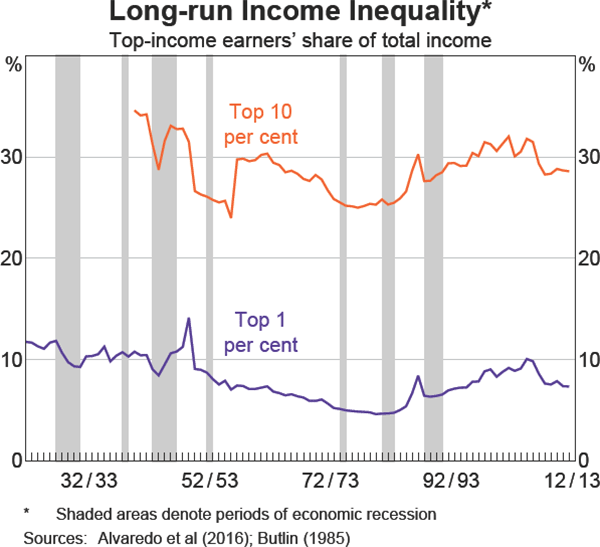
Changes in the state of the economy can have different effects on earners in different parts of the income distribution and thus have the potential to affect income inequality. Historically, the relationship between economic activity and income inequality (as measured by the income shares of top earners) is somewhat unclear for Australia. A visual inspection of the long-run series of income inequality suggests that there is not a strong correlation between fluctuations in economic conditions and income inequality (Graph 1). During recessions in Australia, the income share of top earners has increased in some cases, while in others it has been steady or declined.[1]
This article uses longitudinal data from the HILDA Survey to further investigate the relationship between economic activity and income inequality in Australia. This work focuses on which income earners are most sensitive to fluctuations in economic conditions by tracking how different individuals' incomes vary with aggregate GDP growth. The correlation between personal income growth and aggregate GDP growth will be referred to as ‘the cyclical sensitivity of income’.
The article also explores which components of income are driving this sensitivity and investigates two potential channels: the ‘labour income’ channel and the ‘capital income’ channel. In the literature, these channels are predicted to have offsetting effects on the distribution of income. During a period of strong economic growth:
- ‘Labour income’ channel – bottom-income groups tend to experience larger increases in employment and larger wage increases than top-income groups, leading to lower income inequality.
- ‘Capital income’ channel – a rise in income from business and financial assets will affect the incomes of top-income earners by more, as individuals in this group are more likely to derive a larger portion of their income from these capital sources. By itself, this will lead to higher income inequality.
The ‘labour income’ channel appears to be the most important channel in other countries, such as the United States (Coibion, Gorodnichenko, Kueng and Silvia 2012). The more even wealth distribution in Australia should weaken the effect of the ‘capital income’ channel making it likely that the ‘labour income’ channel is also the most important channel in Australia for influencing the income distribution.
Identifying whether individuals at the top, middle or bottom of the income distribution are more exposed to economic conditions, and through which channels, can help us to understand which groups in the economy are most affected by macroeconomic fluctuations.[2]
Examining how the distribution of income growth responds to changes in economic activity can also help improve our understanding of patterns in aggregate household spending.[3] For instance, cyclical (temporary) changes in income will have a larger effect on aggregate household spending if income growth is mostly concentrated among individuals whose spending is constrained by their current income. These ‘liquidity-constrained’ individuals typically have a relatively high marginal propensity to consume out of temporary income changes (Kaplan, Violante and Weidner 2014).[4] Such analysis is also useful for understanding the causes of short-term changes in income inequality. Previous Australian research has mainly focused on long-run trends in income inequality.[5]
Data
Individual-level data are obtained from the HILDA Survey and cover the period from 2001 to 2014. Two main samples are used for the analysis:
- an ‘employed’ sample – comprising all persons in the survey between the ages of 25 and 60 years who reported a positive wage income in the previous period
- a ‘full’ sample – containing all responding individuals in the survey.[6]
For both samples, the sensitivity of three key income variables to aggregate GDP growth is estimated: total annual income; ‘labour’ or wage & salary income; and ‘capital’ income. Capital income includes: business income, interest from savings & investments, dividends from shares, superannuation, rental income and royalties.[7]
Total income includes labour income, capital income, government payments and ‘other’ income.[8]
Following Mian and Sufi (2016), individuals in each sample are sorted into five income buckets or ‘quintiles’ according to their level of total annual income in the previous year, rather than the current year, so that an individual's position in the income distribution is measured before any growth in their income has occurred over the period.
Table 1 reports summary statistics on the key characteristics for the top and bottom income quintiles of the full sample. Compared with the bottom quintile, top-income earners are more likely to be male, have tertiary qualifications, be self-employed and hold financial assets, though labour income still represents the largest portion of their total income. By comparison, bottom-income earners are more likely to be employed casually or under a fixed-term arrangement. Individuals in this group derive most of their income from labour income and government payments, though capital income still accounts for around 14 per cent of total income.
It is instructive to examine how the incomes of top and bottom earners changed in response to the 2008–09 economic downturn. The response is measured by comparing how the different income components (labour, capital and government payments) contributed to the overall change in real total annual income for individuals in the top and bottom income quintiles over this period (Graph 2).
| Bottom income quintile |
Top income quintile |
Total | |
|---|---|---|---|
| Age (years, mean) | 37 | 45 | 44 |
| Male (%) | 38 | 70 | 49 |
| Tertiary education (%) | 26 | 76 | 48 |
| Self-employed (%) | 5 | 17 | 9 |
| Holds financial assets (%) | 25 | 60 | 40 |
| Casual or fixed-term contract (%) | 24 | 11 | 17 |
| Total annual income ($, mean) | 13,000 | 111,000 | 47,000 |
| Of which: | |||
| Labour income (%) | 41 | 78 | 55 |
| Capital income | 14 | 16 | 15 |
| Business | 3 | 7 | 5 |
| Interest | 4 | 2 | 3 |
| Dividend | 2 | 4 | 2 |
| Other capital(b) | 5 | 3 | 5 |
| Government payments (%) | 41 | 3 | 27 |
| Other income (%)(c) | 4 | 3 | 3 |
|
(a) All amounts are reported in September 2014 dollars; income groups
are determined separately for each year Sources: Author's calculations; HILDA Release 14.0 |
|||
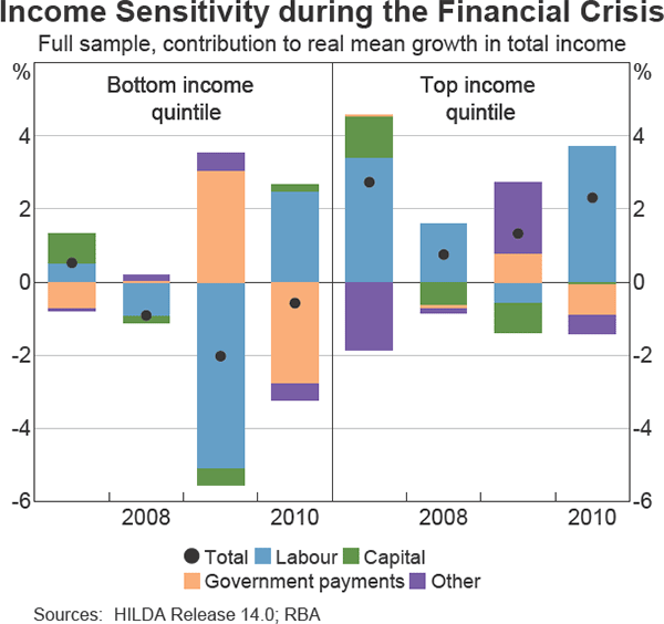
Labour income decreased for the bottom income quintile in 2008 and 2009, although the fall in average labour income for this group was partially offset by government bonus payments received around this time. In contrast, labour income for individuals in the top income quintile experienced only a small decline in 2009. Growth in total annual income slowed, but remained positive, for the top income quintile over the 2008–09 period, although capital incomes did decline.
Together, these patterns provide evidence for both the ‘labour income’ and ‘capital income’ channel in Australia. The response of labour income is more important for those at the bottom of the income distribution, while income from other sources, such as capital assets, seems more responsive for top-income earners.
This is explored in the next section over a longer time period, using regression analysis to control for other determinants of personal income growth. The panel dimension of the HILDA Survey is used to account for compositional change in the individuals who represent the top and bottom income quintile each year.
Model Results
An econometric model is used to estimate the sensitivity of personal income growth to aggregate GDP growth across the different income quintiles, and to decompose the response into a ‘labour income’ and ‘capital income’ effect. The model, discussed in more detail in Appendix A, is estimated separately for total income, labour income and capital income on both the full and employed samples.
To test for the ‘labour income’ channel in Australia, the sensitivity of labour income to GDP growth is measured. The nature of the response is also considered. Labour income is affected by economic fluctuations through individual movements into or out of employment, through a change in hours worked by employed individuals or through changes in wage rates (Bishop and Plumb 2016). In particular, the response of labour income is compared for the full and employed samples, noting that the sensitivity of labour income for the employed sample will only show how much of the response occurs through an adjustment in wage rates or hours worked.
The existence of the ‘capital income’ channel for Australia is then assessed by examining how the sensitivity of capital income to GDP growth varies across income groups and by exploring which components of capital income are most sensitive. Assessing whether the labour or capital income response to GDP growth has a larger effect on the overall response of total income will provide evidence for which channel has a stronger effect in Australia.
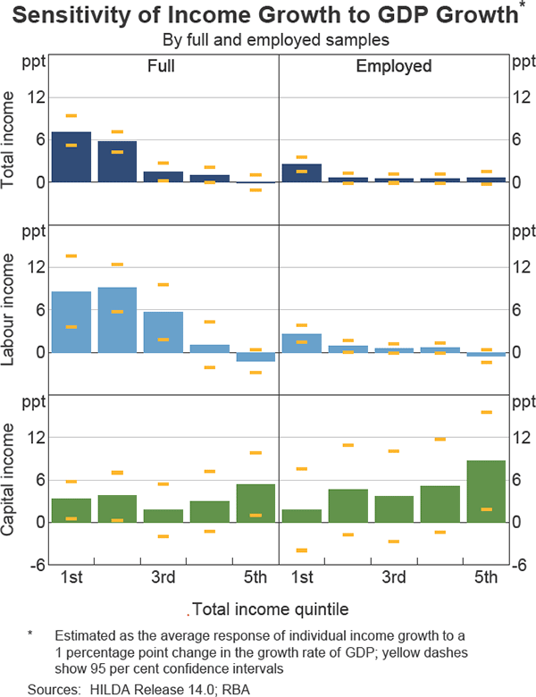
Profiles of cyclical sensitivity are presented for each income variable for both the full and employed samples in Graph 3. These estimates represent the average response of individuals' income growth to a 1 percentage point change in the growth rate of GDP, for each income quintile. For example, for the bottom quintile in the full sample, a 1 percentage point increase in the growth rate of GDP is associated with a 7 percentage point increase in the growth rate of total income.
‘Labour income’ channel
For the full sample, there is a positive and statistically significant relationship between GDP growth and growth in total income and labour income for individuals in the bottom three income quintiles (Graph 3). Labour income is more responsive than total income for these groups, which suggests that insurance mechanisms such as government benefits and transfers play a role in offsetting some of the wage risk faced by bottom-income earners.
In contrast, the sensitivity of total and labour income for the bottom quintiles of the employed sample are more similar, suggesting that low-wage workers receive less of a buffer against aggregate shocks through government payments. More generally, the results for the employed sample show that total and labour incomes of individuals who remain employed from one year to the next in the second and middle quintiles are no longer as sensitive to GDP growth (Graph 3). However, some sensitivity remains for the lowest-income earners, with the bottom income quintile being the only quintile with a sensitivity estimate significantly different from zero.
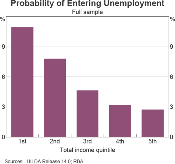
This suggests that most of the sensitivity of income for the bottom- and middle-income groups of the full sample is likely to occur due to transitions into and out of employment, as individuals in these groups have a higher probability of entering into unemployment (Graph 4).[9] For these groups, a 1 percentage point increase in the growth rate of GDP is associated, on average, with a 5 percentage point increase in the growth rate of total income.
For the employed sample, the higher sensitivity of labour and thus total income for the bottom quintile represents the response that occurs through an adjustment in wages or hours worked by individuals in this group. This result may reflect the fact that the bottom income quintile also has a higher share of individuals in casual, fixed-term or part-time employment. There is more scope to increase hours worked for these workers than for full-time workers. The estimates imply that 1 percentage point increase in the growth rate of GDP results in a 2 percentage point increase in the growth rate of total income, on average, for those in the bottom income quintile.
These results provide support for the ‘labour income’ channel in Australia. They suggest that labour income is most responsive to GDP growth for households at the bottom of the income distribution as individuals in bottom-income groups are more exposed to changes in employment status and to an adjustment in hours or wages.
‘Capital income’ channel
For capital income, there is a positive and statistically significant relationship between income growth and GDP growth for the top quintile of both the full and employed samples (Graph 3). Capital income in the top quintile is slightly more sensitive to GDP growth in the employed sample, which could be because employed individuals are more willing to hold riskier, more sensitive assets than those at the extremes of the working life cycle.
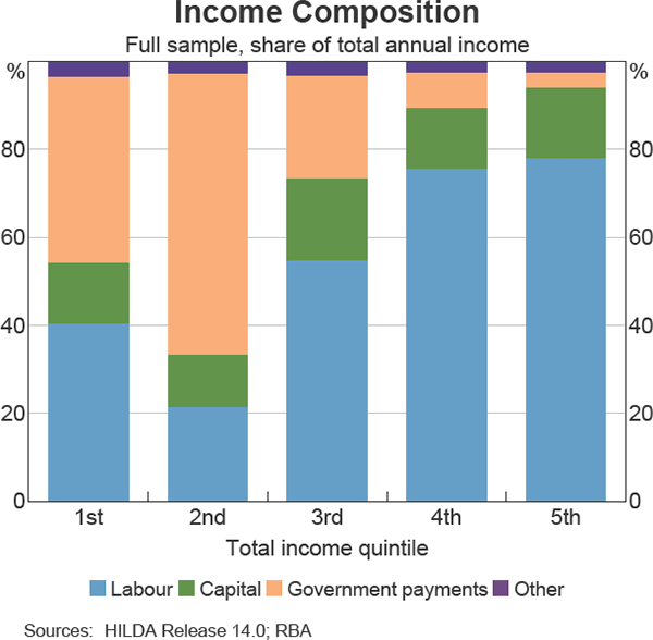
The fact that the high sensitivity of capital income to GDP growth for top-income groups in both samples does not have a large effect on total income is likely to be because of the small share of capital income for most individuals in these groups, of around 13 per cent of total income (Graph 5). A closer look at the income composition of individuals in the top quintile suggests that the procyclical relationship for this group is driven by the highest-earning individuals, because the capital share of total income in the top quintile increases as income rises.
Capital income is also responsive to GDP growth for bottom-income earners in the full sample. The relationship is statistically significant for the lowest two income quintiles of the full sample, which reflects the fact that bottom-income individuals earn some interest income on savings accounts and that retirees derive more income from capital sources (retirees account for around 30 per cent of individuals in the bottom two income quintiles, compared with less than 10 per cent of the top three quintiles).
The sensitivity of capital income in the bottom two income quintiles is not significantly different from zero in the employed sample, suggesting that the sensitivity of retirees' capital income is a driver of the significant outcomes for the full sample.
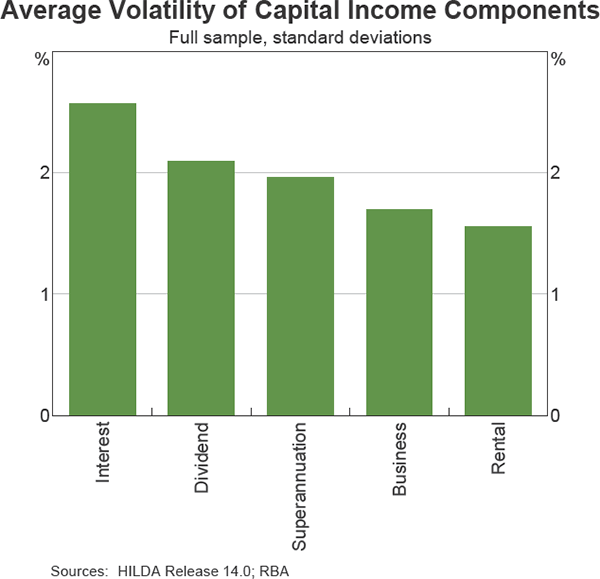
To assess which components of capital income are driving the sensitivity for the top and bottom income quintiles, the average volatility of different capital income components are estimated. Based on this, it appears that interest and dividend earnings are the more volatile sources of income (Graph 6).
To explore this further, the econometric model is re-estimated for capital income, excluding a different capital income component each time. The model is estimated on the full sample to also understand what is driving the sensitivity of capital income that is observed for the bottom income quintiles in Graph 3. Results from estimating these models are shown in Table 2.
For the bottom income quintile, the responsiveness of capital income is most affected when the interest income component is excluded (Table 2, column 2). The coefficient on GDP growth decreases and is no longer statistically significant. There is also a large decrease in the coefficient for the second income quintile, which is the income group that contains the highest share of retired individuals. This suggests that the sensitivity of capital income for bottom-income earners may be driven by the high share of interest income in total capital income for retirees.
In contrast, it appears that all components of capital income contribute to the sensitivity for the top income quintile. This may be because individuals in this group tend to hold more diversified asset portfolios. However, the coefficient on GDP growth increases when business income is excluded, suggesting that most of the sensitivity to capital income for the top quintile occurs through income from financial assets, such as dividend and interest income.
These results provide evidence that the ‘capital income’ channel is operating in Australia, although somewhat differently than it does in the United States. Rather than capital income playing a role solely for top-earning individuals, capital income is procyclical at both the top and bottom of the income distribution in Australia. However, the response of capital income is much higher for the top-income group and is driven mainly by changing returns to financial assets, rather than by business or rental income.
Comparing the profiles of total, labour and capital income also shows that labour income appears to be the component of income driving the overall sensitivity for total income. This provides evidence that the ‘labour income’ channel is more potent for Australia.
Conclusion
This article examines how the effect of changing economic conditions on income growth varies across different income groups and different income components. Results suggest that labour income is most sensitive at the bottom of the income distribution as those households are more exposed to unemployment and to adjustments in hours worked and/or wages. Capital income is responsive to GDP growth for those in the top and bottom income quintiles; however, capital income is much more sensitive for the top income quintile and is driven mainly by changing returns to financial assets.
| Total income quintile | Total capital |
Interest |
Excluding: Dividend |
Business |
|---|---|---|---|---|
| Bottom | 3.3*** | 0.5 | 3.1* | 3.2** |
| 2nd | 3.8*** | 0.8 | 2.3** | 3.5** |
| 3rd | 1.8 | 2.3 | 1.5 | 2.4 |
| 4th | 3.0 | 0.4 | 1.0 | 4.9 |
| Top | 5.4**** | 5.1*** | 4.6** | 5.8*** |
| Observations | 154,836 | 154,836 | 154,836 | 154,836 |
|
(a) *, ** and *** indicate statistical significance at the 10, 5 and 1 per cent levels, respectively; all regressions include a set of control variables for individuals' circumstances, as well as state and industry fixed effects Sources: Author's calculations; HILDA Release 14.0 |
||||
These effects provide evidence for both a ‘labour income’ channel and a ‘capital income’ channel in Australia. The two channels have partly offsetting effects on inequality, but the response of labour incomes appear to have the stronger effect for Australia. This suggests that changes in economic conditions will have a more pronounced effect on bottom-income groups, which implies that stronger economic conditions tend to reduce income inequality in Australia, and vice versa.
Appendix A: The Model
The econometric model used to estimate the sensitivity of personal income growth with respect to aggregate GDP growth is shown by Equation A1. The model chosen is based on the empirical models of Guvenen, Kaplan and Song (2014) and Cervini-Plá, López-Villacivencio and Silva (2015), and draws upon an extensive wage cyclicality literature. This model is estimated separately for total, labour and capital income on both the full and the employed samples. Individuals in each sample are grouped into five buckets (or quintiles) according to their level of income.
The model is specified as:
where Δln (Yi,t) is the change in the log of the income variable
of interest (total, labour and capital income) from year t−1
to
t for individual i. The term  is a dummy variable
equal to one if individual
i is in quintile q at year t−1. A dummy
variable is included for each income quintile to control for differences
in average income growth across quintiles.
The term Δln (GDPt) is the change in log GDP from t−1 to t. This variable is interacted with the income quintile dummies and the coefficients on these interaction terms βq provide measures of the response of income growth to GDP growth for each income quintile.
The model also includes a set of variables that are likely to be important determinants of income growth rates across individuals. These ‘control’ variables (CONTROLSi,t) include individual-level circumstances such as age (and age squared), gender, years of education, marital status and migrant status, as well as industry and state fixed effects. Like the income quintile groups, individuals' characteristics are measured at time t−1 so that their effect on subsequent income growth can be estimated.
The separate models for each income variable and for each sample are estimated using robust standard errors, clustered at the individual level. This accounts for possible heteroskedasticity and serial correlation of an individual's income shocks over time, but does not adjust for potential bias introduced by any cross-sectional correlation between the income shocks of different individuals in the same income quintile.
Footnotes
This work was completed within Economic Research Department. [*]
A recession is defined prior to 1960 as one year of negative GDP growth using annual data from Butlin (1985). After 1960, the three recessions shaded in the graph are the ones identified by Gillitzer, Kearns and Richards (2005) using coincident indices. [1]
A related literature looks at the distributional effects of changes in monetary policy. See Coibion et al (2012) and Hughson et al (2016), for example. [2]
Recent studies also examine how income and consumption growth are affected by changes in the distribution of wealth caused by changing economic conditions, wtih particular focus on housing assets. See Mian and Sufi (2016) and Krueger, Mitman and Fabrizio (2016), for example. [3]
Kaplan et al (2014) find that around 20 per cent of households in Australia are liquidity-constrained or ‘hand to mouth’ and spend all of the regular inflow of income they receive each pay period. [4]
See, for example, Fletcher and Guttmann (2013); Greenville, Pobke and Rogers (2013); and Dollman, Kaplan, La Cava and Stone (2015). [5]
An unbalanced panel allows for individuals to exit and re-enter the sample, but respondents must be present for at least two consecutive waves of the survey to be able to calculate growth rates for income. [6]
A more complete definition of capital income might also include realised capital gains and net-imputed rent for owner-occupiers. While net-imputed rent can be approximated, neither of these variables are measured directly in the HILDA Survey. [7]
All income variables are converted to real terms using the consumer price index. ‘Other’ income includes private transfers, foreign pensions, child support payments, scholarships, workers compensation, inheritance and other irregular payments. Government payments income is defined as the gross amount of pensions and allowances received, and is not reported net of taxes. [8]
The probability of entering into unemployment is calculated by tracking individuals over time and calculating the share of individuals who were employed in each income quintile at time t and transitioned into unemployment at time t + 1. [9]
References
Alvaredo F, A Atkinson, T Pikkety, E Saez and G Zucman, ‘The World Wealth and Income Database’. Available at <http://www.wid.world/>, viewed 26 September 2016.
Bishop J and M Plumb (2016), ‘Cyclical Labour Market Adjustment in Australia’, RBA Bulletin, March, pp 11–20.
Butlin N (1985), ‘Australian National Accounts: 1788–1983’, Australian National University Source Papers in Economic History 6.
Cervini-Plá M, A López-Villacivencio and J Silva (2015), ‘The Heterogeneous Cyclicality of Income and Wages Among the Distribution’, Groupe d’Analyse et de Théorie Economique (GATE) 1506.
Coibion O, Y Gorodnichenko, L Kueng and J Silvia (2012), ‘Innocent Bystanders? Monetary Policy and Inequality in the U.S.’, IMF Working Paper WP/12/199.
Dollman R, G Kaplan, G La Cava and T Stone (2015), ‘Household Economic Inequality in Australia’, RBA Research Discussion Paper No 2015-15.
Fletcher M and B Guttmann (2013), ‘Income Inequality in Australia’, Economic Roundup, 2, pp 35–56.
Gillitzer C, J Kearns and A Richards (2005), ‘The Australian Business Cycle: A Coincident Indicator Approach’, RBA Research Discussion Paper No 2005–07.
Greenville J, C Pobke and N Rogers (2013), ‘Trends in the Distribution of Income in Australia’, in Productivity Commission Staff Working Paper, Productivity Commission, Canberra.
Guvenen F, G Kaplan and J Song (2014), ‘How Risky are Recessions for Top Earners’, American Economic Review: Papers and Proceedings, 104(5), pp 148–153.
Hughson H, G La Cava, P Ryan and P Smith (2016), ‘The Household Cash Flow Channel of Monetary Policy’, RBA Bulletin, September, pp 21–29.
Kaplan G, G Violante and J Weidner (2014), ‘The Wealthy Hand-to-Mouth’, Brookings Papers on Economic Activity, 1, pp 77–153.
Krueger D, D Mitman and P Fabrizio (2016), ‘Macroeconomics and Household Heterogeneity’, National Bureau of Economic Research) (NBER) Working Paper 22319.
Mian A and A Sufi (2016), ‘Who Bears the Cost of Recessions? The Role of House Prices and Household Debt’, NBER Working Paper 22256.
