Bulletin – June 2014 Australian Economy The Rise in Household Saving

Introduction

Between the early 1970s and the early 2000s, the aggregate household saving ratio in Australia declined steadily, from around 20 per cent to around zero (Graph 1). This trend was driven by a number of factors, including an increased availability of credit, falling real interest rates, more stable economic outcomes and rising asset prices, while changes in household income growth and expectations may also have affected the dynamics of the saving ratio over a run of years.^[1] The importance of these various factors waxed and waned over the three decades, but it is likely that all contributed to some extent to a higher rate of growth in consumption compared with income, and so to the fall in the saving ratio.

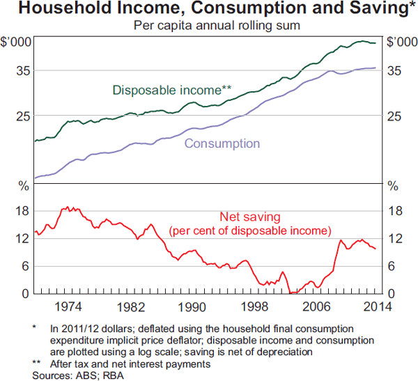
However, the household saving ratio reversed much of this decline between 2006 and 2010, reflecting both an increase in growth of disposable income and a slowing in consumption growth. The saving ratio is now at a level similar to that of the mid 1980s. This is an important change in household behaviour, particularly given that household consumption accounts for a little more than half of GDP.

As argued in Browning and Lusardi (1996), it is difficult to draw firm conclusions from aggregate data about what drives household saving behaviour. For that reason, this analysis uses household-level data from the 2003/04 and 2009/10 Household Expenditure Surveys (HES) to examine the saving behaviour of various household types. The HES are cross-sectional surveys of a nationally representative sample of households in Australia and detail household income and expenditure, as well as a range of socio-demographic characteristics.^[2]

The period between 2003/04 and 2009/10 saw rapidly rising asset prices and strong economic growth, as well as the global financial crisis and times of rising unemployment. The average age of the population rose gradually throughout this time. By considering how the saving behaviour of different households changed, we aim to understand the relative importance of household income, credit constraints, precautionary motives, household wealth and life-cycle factors for saving. To do this, the relationships between saving and various household characteristics that are correlated with these drivers are examined. For example, to the extent that saving varies with household characteristics that are deemed to indicate a higher degree of income risk, we draw the inference that this underlying risk factor has played a role in driving saving behaviour, although this is not conclusive because we cannot measure this risk factor directly.^[3]

Descriptive Analysis

The distribution of household saving is first examined to see how saving varies between different household groups, and whether certain types of households increased their saving by more than others between 2003/04 and 2009/10.

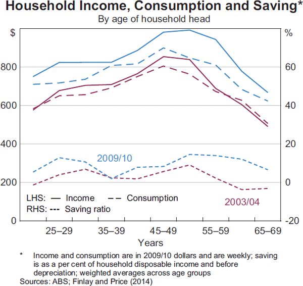
Household consumption and income follow a broadly similar pattern over the life cycle (Graph 2). The increase in consumption around middle age suggests that households do not fully smooth their consumption, although Attanasio (1999) points out that the hump-shaped consumption profile is less pronounced after controlling for family size and composition. Between the 2003/04 and 2009/10 HES, saving increased for younger and older households in particular, with the increase in consumption lagging behind the increase in income for these groups.

Wealthier households tend to save more, although changes in household saving behaviour do not appear to be specific to any particular level of household wealth, with the saving ratio increasing across all wealth quintiles between 2003/04 and 2009/10 (Graph 3).^[4] Similarly, saving increases with age-matched income quintiles, and, as with wealth, most age-matched income quintiles saw a rise in saving between 2003/04 and 2009/10, with only the lowest income group recording a fall (Graph 4).^[5]

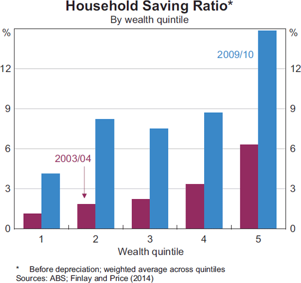
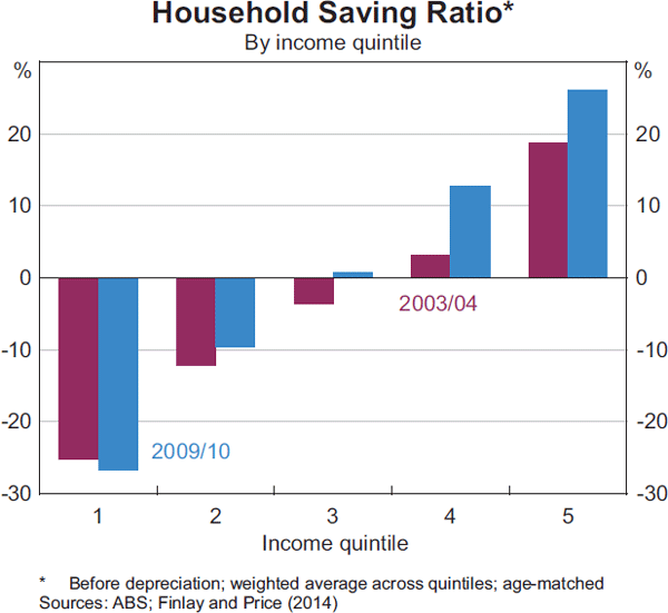
This simple descriptive analysis suggests that relatively young and old households, but not middle-aged households, increased their saving considerably between 2003/04 and 2009/10, while an increase in saving was evident across most wealth and income groups.

Cross-sectional Analysis

While the descriptive analysis gives a sense of which household types are saving the most, and how their saving has changed over time, it does not control for other factors pertinent to the saving decision. Turning to a more comprehensive approach to identify the determinants of saving behaviour, this section presents the results from a model of what influences the median household's saving ratio at a point in time.^[6] The potential determinants of saving behaviour considered in the model, and their effect on saving, are discussed below.

Household income

Income is a particularly important determinant of household saving, although there is some debate as to how it affects saving. Our results are estimated under the assumption that it is the deviation of a household's current level of income from its permanent or long-run level of income that affects saving, although the results are robust to relaxing this assumption. In particular, a household's saving ratio is modelled as:

Here y_i is the natural logarithm of household i 's current income, is the logarithm of permanent income, and X_i represents other household characteristics pertinent to the saving decision such as age, employment status and the composition of a household. This model implies that a household will increase its saving ratio if its current level of income rises by more than its permanent level of income, for example due to an unexpected one-off bequest. Conversely, a household will reduce its saving ratio if its current level of income falls by more than its permanent level of income, for example due to a temporary spell of unemployment.

In practice, the permanent income of a household cannot be observed. Instead, it is modelled as the fitted value from a regression of current income on household characteristics that affect permanent income. This implies that the average deviation of current income from modelled permanent income across all households is zero; modelled permanent income will also fail to capture any changes in households' future income expectations. Also included in the model is the household head's level of education; educational attainment is often regarded as a good proxy for permanent income, and, importantly, it is likely to be correlated with households' future income expectations.^[7]

As expected, households whose current level of income is above their permanent level of income tend to save more than otherwise similar households would; the effect of education on saving is mixed across the two sample periods.

Credit constraints

Credit constrained households are identified from households' responses to questions regarding financial stress; households are assumed to be credit constrained if they answer in the affirmative to at least two out of seven financial stress questions. An increase in the incidence of credit constraints would be expected to lift household saving, since some households that may wish to borrow to fund consumption would be unable to do so and so would consume less than otherwise; credit constrained households must also save in order to fund large purchases, rather than being able to borrow to make the purchase.^[8] In accordance with this, we find that households that are financially constrained tend to have higher saving ratios, holding all else equal.^[9]

Precautionary motives

Households that save in case of an unforeseen need for money are said to be saving for precautionary motives. Theory predicts that households that face a relatively high risk of unforeseen increases in expenditure or reductions in income will save more than other households, all else equal (see, for example, the models outlined in Zeldes (1989), Deaton (1991) and Carroll, Hall and Zeldes (1992)).

In our model, precautionary motives are captured by variables that describe households with relatively less secure incomes or those who are relatively more vulnerable to income shocks, such as migrant and single-parent households, as well as variables that describe households that are vulnerable to an asset price shock, such as self-funded retirees. Our results suggest that people do save for precautionary reasons, with those households that are more likely to face future income shocks, or are less resilient to such shocks, tending to save more than other households.

Household wealth

Higher wealth has been found to have a significantly positive effect on household consumption in Australia, and therefore a negative effect on saving (Dvornak and Kohler (2003); Yates and Whelan (2009); Windsor, Jääskelä and Finlay (2013)).

Our results suggest that, overall, higher wealth-to-income ratios are associated with lower saving ratios (and therefore more consumption). In general, this wealth effect is smaller for the oldest households, which is consistent with Windsor et al (2013), who interpret this as evidence against a traditional wealth effect on consumption. Rather, they suggest that rising household wealth increases consumption by reducing liquidity constraints, which are more likely to be binding on the young than the old.

Owning a dwelling outright tends to be associated with higher saving for younger households and lower saving for older households. For younger households, this effect may be capturing personal preferences rather than wealth, with those who own their home outright early in their working lives being inherently diligent savers. For the older age groups, owning a home is likely to be associated with a higher degree of financial security, reducing the need to save in case of emergency. Regarding debt, our results suggest that the more debt a household has relative to their assets, the less the household saves.

Life cycle

Perhaps unsurprisingly, after controlling for other household characteristics, pre-retirement households (those aged 50 to 64 years) are found to save more than middle-aged households (30 to 49 years), who in turn save the same or more than the youngest households (less than 30 years). Older households tend to save more than younger households would, were they to face similar living circumstances, perhaps due to bequest motives or precautionary saving given an uncertain life expectancy. This suggests that the low level of saving by older households that is evident in the data is predominantly due to their circumstances rather than their age.

The Rise in Saving between 2003/04 and 2009/10

We now turn to the question of what drove the change in saving behaviour between 2003/04 and 2009/10. Graph 5 presents a model-based decomposition of the total change in the saving ratio into changes in households' propensity to save given particular household characteristics (captured by changes in estimated model parameters between the two surveys) and changes in household characteristics.^[10] The model used is very similar to that of the previous section, except that it is applied to the mean saving ratio rather than the median saving ratio.^[11] Strikingly, the decomposition suggests that changes in the characteristics of households across the two time periods played virtually no role in the increase in household saving between 2003/04 and 2009/10, with changes in model parameters (red bar on the left of Graph 5) accounting for all of the increase.

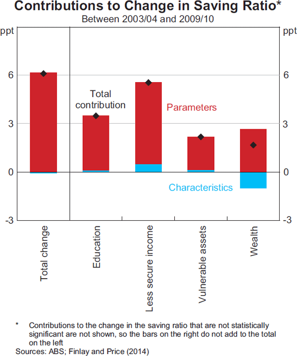
As well as the estimated total contribution, Graph 5 also shows the contribution from changes in model parameters and household characteristics related to: households' level of education; the extent of their precautionary motives (split into those related to incomes and those related to assets); and household wealth.

Income

The income variable that we employ (the deviation of current income from modelled permanent income) does not contribute to the increase in the saving ratio between 2003/04 and 2009/10, since by construction the average deviation of temporary income from modelled permanent income is zero in both surveys.^[12]

A change in saving behaviour associated with the household head's level of education does contribute to the increase in the overall saving ratio, however. We find that more educated households increased their propensity to save relative to other households between 2003/04 and 2009/10, with this increase largest for the most highly educated households. If education is interpreted as a proxy for permanent income, or equivalently for expectations regarding future increases in income, then the rise in saving for more educated households suggests a downward reassessment by these households of their future income prospects relative to their current income, possibly driven by the financial crisis.

Precautionary motives

We find that those households who appear to have less secure income or are more vulnerable to an asset price shock increased their saving between 2003/04 and 2009/10. This is consistent with a greater degree of risk aversion, or a greater degree of risk, for households with these characteristics.

Household wealth

Wealthy households tended to increase their saving between 2003/04 and 2009/10, suggesting an effort to rebuild wealth after the effects of the financial crisis. This was also true of households with high debt levels, which may indicate that attitudes to debt had changed, or that the transition to higher debt levels (starting from the late 1980s or early 1990s) had run its course.

Life cycle

With the exception of pre-retirement aged households (which is one of the set of household characteristics suggestive of being vulnerable to asset price shocks in Graph 5), saving behaviour associated with household age was not found to change significantly between 2003/04 and 2009/10.

Summary of results

In summary, the results from this analysis are consistent with a number of factors driving the increase in household saving between 2003/04 and 2009/10. The rise in saving for those groups judged to be vulnerable to income or asset price shocks is consistent with precautionary motives playing a role, with households observing and responding to events overseas, as well as rising unemployment and declines in asset prices domestically. Related to this, the rise in saving for those with high debt levels is consistent with households adopting a more prudent attitude towards debt over this period, or the transition to higher debt levels having run its course. The rise in saving for more educated households is consistent with a downward reassessment of expected future income prospects for these households. Finally, the rise in saving for wealthy households is consistent with a reassessment of expected future capital gains and a desire to rebuild wealth, with declines in asset prices following the global financial crisis both reducing wealth immediately and reminding households that asset prices can fall as well as rise. However, since household preferences cannot be directly measured, we can only draw inferences based on which household groups changed their propensity to save, and other interpretations of the data are possible.

Implications of Ageing on Household Saving

Although the ageing of the population does not appear to have played a significant role in the change in the aggregate household saving ratio between 2003/04 and 2009/10, life-cycle factors remain an important factor in household saving behaviour. In 2009/10, the oldest people in the large baby boomer cohort were nearing retirement age (65 years).^[13] Given older households save less than middle-aged households, the baby boomer cohort transitioning from middle age to retirement may place downward pressure on the aggregate saving ratio in the future.^[14]

To estimate the possible future impact of the ageing of the population on household saving, the estimated effects on saving of the age of a household head and their year of birth are combined with population projections from the Australian Bureau of Statistics (ABS 2013).^[15] The results suggest that the ageing of the population has subtracted around half a percentage point from the aggregate household saving ratio since 2009/10; over the next 15 years, ageing is expected to subtract a further 2 percentage points. While these effects are non-trivial in aggregate, they are relatively small in any given year and small relative to actual movements in the saving ratio.^[16]

Conclusion

We find that the important determinants of household saving behaviour are consistent with theory and previous findings. As might be expected, households' saving ratios tend to increase with income, while saving is found to decrease with wealth and gearing. Financially constrained households and households deemed to be at risk of a future income shock tend to save more than other households, all else equal. While saving differs substantially across age groups, we find that, at least in part, this reflects differences in other features of these groups.

The rise in household saving from 2003/04 to 2009/10 appears to have been driven by changes in saving behaviour associated with certain household characteristics, rather than changes in particular characteristics. The results suggest that the large increase in household saving over that period was underpinned by precautionary saving motives, a reduction in expected future income gains for more educated households and an effort to rebuild wealth after the financial crisis. Changing attitudes to debt (or the transition to higher debt levels having run its course) may have played a role. This suggests that if memories of the financial crisis fade, and asset prices and the appetite for risk increases, one might expect household saving to fall; conversely, if households' reduced expectations of future income gains persist, higher saving may be more enduring.

Finally, while the ageing of the population does not appear to have played a significant role in changes in the saving ratio between 2003/04 and 2009/10, it may place mild downward pressure on the saving ratio over coming years.

Appendix A: Median Regression Results

Table A1: Median Model of Household Saving Ratio – Regression Results^(a)

Coefficients

Variable	2003/04	2009/10	Difference over time
Income	0.6***	0.6***	0.0
Education
– TAFE/certificate	−2.6	3.2*	5.8**
– University	−4.3**	4.3**	8.6***
Single-parent household	−3.1	8.4***	11.5**
Government income (>20%)	8.6***	14.5***	5.8*
Financially constrained	4.0*	3.7	−0.4
Risk of unemployment	1.9	0.1	−1.8
Non-English-speaking migrant	6.2***	7.4***	1.2
Self-funded retiree	−13.6***	−1.5	12.1**
Wealth-to-income ratio
– Young	−0.4	−0.5	−0.1
– Middle-aged	−0.3**	−0.5***	−0.2
– Pre-retirement	−0.4***	−0.1	0.4**
– Old	−0.2**	−0.2***	−0.1
Own a home
– Young	8.3	9.0	0.8
– Middle-aged	3.3	5.9	2.6
– Pre-retirement	−6.8*	−4.2	2.6
– Old	−12.7**	−3.5	9.2
Gearing ratio
– Young	−9.0**	0.9	9.9*
– Middle-aged	−10.1	−7.7	2.3
– Pre-retirement	−17.0	−1.7	15.3
– Old	−19.6	−11.6	8.0
Young (<30)	−5.1	−2.4	2.7
Pre-retirement (50–64)	9.6***	7.8**	−1.8
Old (≥65)	6.7	4.6	−2.1
(a) ***, ** and * represent significance at the 1, 5 and 10 per cent level, respectively; HES household weights used; 500 repetitions of bootstrapped weights are used to obtain the standard errors; reference household is a single middle-aged male, born in an English-speaking country, not financially constrained, same or better standard of living compared with a year ago, working in a high-skilled occupation, with high school as highest level of education and lives in urban New South Wales Sources: ABS; Finlay and Price (2014)

Footnotes

The authors are from Economic Analysis Department. This article draws extensively on Finlay and Price (2014). [*]

See, for example, Stevens (2011) for a discussion of some of these factors. [1]

The 2003/04 HES surveyed around 7,000 households, while the 2009/10 HES surveyed around 10,000 households. The sample of households used in this article excludes those who give zero or negative values for income, and households where the household head is aged over 75 years. Households in the top and bottom 2 per cent of the saving ratio distribution are also excluded from the sample to minimise the impact of potentially erroneous responses. [2]

While other studies have used household-level data to analyse household saving behaviour in Australia (see, for example, Harris, Loundes and Webster (2002) and Berger-Thomson, Chung and McKibbin (2009)), they do not address the rise in the household saving ratio over the 2000s. [3]

Note that after controlling for other important variables such as income, education level and age, saving falls with wealth. [4]

Age-matching controls for age-related effects when comparing income quintiles. For example, since post-retirement households are typically in the lower income quintiles, the saving behaviour of older households will have a significant influence on the saving behaviour of the lower (non age-matched) income quintiles. Age-matching is done by splitting the households in each age group into separate income quintiles. Income quintiles from each age group are then recombined, so that, for example, the lowest age-matched income quintile consists of all those households that make up the lowest income quintile within each age group. [5]

See Appendix A for a table of model estimates. Note also that the median saving ratio gives a better indication of how much a ‘typical’ household saves compared with the mean saving ratio, which can be heavily influenced by a small number of outliers. The mean saving ratio is nonetheless important since it determines economy-wide household saving, and will be considered below when we examine what drove the change in saving behaviour between 2003/04 and 2009/10. [6]

Education is widely used as a proxy for permanent income; Attanasio and Weber (2010), for instance, document that more educated households tend to have steeper income profiles than those headed by less educated individuals. [7]

Note, however, that these explanations should only affect a household's saving rate in a transition to being more or less credit constrained, with the long-run rate of saving unaffected. [8]

Note that in our model we only capture households that are currently credit constrained. In an overlapping generations framework, Connolly and Kohler (2004) and Kent, Ossolinski and Willard (2007) show that the adjustment to a new equilibrium following a change in credit constraints can take many years to complete. As such, the lowering of credit constraints that occurred in the late 1980s and early 1990s may still have been affecting household behaviour during our sample period. In particular, with a decline in the number of households who purchased housing during the earlier period of elevated credit constraints and relatively low house prices, there will be a decline in the share of households that are likely to experience very large capital gains on selling their homes (and who therefore need to save less than otherwise similar households). [9]

The model-implied mean saving in year i  can be expressed as

View MathML

where describes household characteristics and describes the estimated effect of those characteristics on saving behaviour. The change in the saving ratio can then be expressed as

View MathML

where the first term captures parameter effects holding household characteristics constant at their 2003/04 level, and the second term captures the effect of changing household characteristics holding model parameters constant at their 2009/10 level, where year 2 represents 2009/10 and year 1 represents 2003/04.

[10]

Finlay and Price (2014) also examine the changes in households' propensity to save using the median regression model discussed in the ‘Cross-sectional Analysis’ section; the results from the median and the mean analyses are similar. [11]

Note that this is a shortcoming of the way the permanent income variable is constructed – in reality, economy-wide deviations of current from permanent income could occur, for example during a temporary terms of trade boom. [12]

A baby boomer is defined as someone born between 1946 and 1964. [13]

Note that the ageing of the population is in part driven by lengthening life expectancy. One might expect this to increase saving among currently working households, given the need to fund more years of retirement, and result in households working later into life, again resulting in higher saving than otherwise. [14]

See Appendix A of Finlay and Price (2014) for more detail. In this scenario, the birth cohort effect for those born after 1995 is assumed to be equal to the birth cohort effect for those born between 1990 and 1995. [15]

Note that these estimates are partial equilibrium in nature; in general equilibrium, lower saving by the relatively large baby boomer cohort in Australia and overseas would be expected to place upward pressure on real interest rates, encouraging other groups to save more. [16]

References

ABS (Australian Bureau of Statistics) (2013), ‘Population Projections, Australia, 2012 (base) to 2101’, ABS Cat No 3222.0, November.

Attanasio OP (1999), ‘Consumption’, in J Taylor and M Woodford (eds), Handbook of Macroeconomics, Volume 1B, Handbooks in Economics 15, Elsevier Science, Amsterdam, pp 741–812.

Attanasio OP and G Weber (2010), ‘Consumption and Saving: Models of Intertemporal Allocation and Their Implications for Public Policy’, Journal of Economic Literature, 48(3), pp 693–751.

Berger-Thomson L, E Chung and R McKibbin (2009), ‘Estimating Marginal Propensities to Consume in Australia Using Micro Data', RBA Research Discussion Paper No 2009-07.

Browning M and A Lusardi (1996), ‘Household Saving: Micro Theories and Micro Facts’, Journal of Economic Literature, 34(4), pp 1797–1855.

Carroll C, R Hall and S Zeldes (1992), ‘The Buffer-Stock Theory of Saving: Some Macroeconomic Evidence’, Brookings Papers on Economic Activity, 1992(2), pp 61–156.

Connolly E and M Kohler (2004), ‘The Impact of Superannuation on Household Saving’, RBA Research Discussion Paper No 2004-01.

Deaton A (1991), ‘Saving and Liquidity Constraints’, Econometrica, 59(5), pp 1221–1248.

Dvornak N and M Kohler (2003), ‘Housing Wealth, Stock Market Wealth and Consumption: A Panel Analysis for Australia’, RBA Research Discussion Paper No 2003-07.

Finlay R and F Price (2014), ‘Household Saving in Australia’, RBA Research Discussion Paper No 2014-03.

Harris MN, J Loundes and E Webster (2002), ‘Determinants of Household Saving in Australia’, Economic Record, 78(241), pp 207–223.

Kent C, C Ossolinski and L Willard (2007), ‘The Rise of Household Indebtedness’, in C Kent and J Lawson (eds), The Structure and Resilience of the Financial System, Proceedings of a Conference, Reserve Bank of Australia, Sydney, pp 123–163.

Stevens G (2011), ‘The Cautious Consumer’, RBA Bulletin, September, pp 77–82.

Windsor C, J Jääskelä and R Finlay (2013), ‘Home Prices and Household Spending’, RBA Research Discussion Paper No 2013-04.

Yates J and S Whelan (2009), Housing Wealth and Consumer Spending, AHURI Final Report No 132, Australian Housing and Urban Research Institute, Melbourne.

Zeldes S (1989), ‘Consumption and Liquidity Constraints: An Empirical Investigation’, Journal of Political Economy, 97(2), pp 305–346.