Bulletin – March 2013 Australian Economy GDP Revisions: Measurement and Implications
- Download the article 1.76MB
Abstract
Gauging economic conditions in real time is challenging, in part because economic data are difficult to measure and subject to subsequent revision as more information becomes available. This article investigates the pattern and size of revisions to real gross domestic product (GDP) over the past decade or so. Revisions to early estimates of GDP can be large and, over the past 15 years, have tended to increase measured growth, although the extent of revision is in line with international experience. This article also examines the feasibility of adjusting real-time estimates of GDP for apparent patterns in revisions, predicting future revisions and calculating confidence intervals around the historical data. The uncertainty around real-time GDP estimates highlights the importance of monitoring a wide range of information when assessing current economic conditions.
Introduction
Assessments of current economic conditions have an important bearing on near-term forecasts of activity and inflation. However, making these assessments in real time is a challenging task for macroeconomic policymakers. One issue is that economic data are difficult to measure and subject to revision as more information is obtained. There is typically a trade-off between timeliness and reliability and so, in order to produce timely estimates, statistical agencies publish data before all information sources are available. As a result, early estimates of many economic aggregates may differ from subsequent, more informed estimates. Gross domestic product (GDP) is one important economic aggregate that is frequently subject to revision, reflecting the large amount of information used in its construction, some of which is not available on a timely basis. GDP measures the total value of final goods and services produced within an economy over a given period of time, and provides a comprehensive summary of the current state of the economy.
In Australia, GDP data are published at a quarterly frequency by the Australian Bureau of Statistics (ABS), around two months after the end of the reference quarter. Real GDP is measured using three different approaches, based on expenditure (GDP(E)), income (GDP(I)) and production (GDP(P)).[1] The ABS considers the average of these three measures (GDP(A)) to be the most reliable estimate of final output, in part because independent errors in the underlying measures are often offsetting (Aspden 1990; ABS 2011). The choice between the available GDP measures in real time would be inconsequential if the discrepancy between them was small. However, typically this is not the case; the range of initial quarterly growth estimates over the past two decades has averaged around half a percentage point (Graph 1).
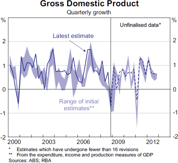
Revisions to GDP are driven by several things. First, they can reflect the incorporation of newly available data, as many data that feed into the national accounts are not available in a timely fashion; for example, some taxation data are only available at an annual frequency from the Australian Taxation Office, whereas initial GDP estimates are published around nine weeks after the end of each quarter. Second, once a year, the ABS undertakes a more detailed reconciliation of each measure of GDP, which generally results in further revisions. Third, regular re-estimation of seasonal patterns, and the rebasing of volume estimates, can also lead to revisions. Finally, revisions can result from methodological changes in the compilation of the national accounts or the correction of errors.
This article examines the extent to which early estimates of GDP are revised, and considers which measure of GDP may give the best read of economic conditions in real time. A range of metrics are employed, such as the average size and direction of revisions for each GDP measure and its components. The article concludes with an assessment of the broader implications of this uncertainty for the presentation and interpretation of real-time GDP data.[2]
Measuring Revisions to GDP Growth
Analysis of revisions is complicated by the fact that ‘final’ estimates are never directly observed because revisions can continue indefinitely. It is necessary, therefore, to make a judgement about when estimates approximate final values. In this article, the ‘final’ value for GDP growth in a given quarter is assumed to be the estimate four years following the initial release, and this ‘final’ value of GDP(A) growth is treated as the best estimate of GDP growth. The analysis in this article draws on initial estimates, that is real-time vintages, of the national accounts, beginning in the September quarter 1998, following the introduction of the 1993 System of National Accounts, and finishing in the December quarter 2008 (leaving four years of data following the end-point to allow the last observation to reach its assumed final value). All analysis is conducted using quarterly or year-ended growth in GDP.
A common metric for assessing the size of revisions is the ‘mean absolute revision’, which measures the average size of revisions regardless of sign (Table 1). Since 1998, the first estimate of growth in GDP(A) has been revised, on average, by more than 0.3 percentage points in quarterly terms and 0.5 percentage points in year-ended terms. To put this into perspective, the average quarterly growth rate of real GDP was 0.8 per cent during this period, with a standard deviation of 0.4 percentage points. The average size of revisions to a particular quarter decreased with subsequent releases, as new data became available and the estimates were refined, but even after three years, quarterly growth estimates of GDP(A) diverged from their ‘final’ values on average by around 0.2 percentage points. In quarterly terms, revisions to early estimates have been largest for the expenditure measure of GDP, while revisions have tended to be smaller for the production measure. This suggests that GDP(P) arguably has been a more reliable indicator of activity in real time than either GDP(E) or GDP(I), in the sense that initial growth estimates of GDP(P) have tended to be closer to ‘final’ growth estimates than for the other measures. In a similar vein, quarterly growth in GDP(P) has historically also been less variable than the other measures of GDP growth, suggesting that it is subject to less measurement error (ABS 2011).
| Initial | One year | Two years | Three years | |
|---|---|---|---|---|
| Quarterly growth: | ||||
| GDP(A) | 0.35 | 0.31 | 0.22 | 0.20 |
| GDP(E) | 0.60 | 0.49 | 0.32 | 0.30 |
| GDP(I) | 0.45 | 0.43 | 0.36 | 0.29 |
| GDP(P) | 0.33 | 0.23 | 0.19 | 0.18 |
| Year-ended growth: | ||||
| GDP(A) | 0.52 | 0.42 | 0.32 | 0.18 |
| GDP(E) | 0.63 | 0.50 | 0.38 | 0.24 |
| GDP(I) | 0.73 | 0.59 | 0.51 | 0.27 |
| GDP(P) | 0.58 | 0.51 | 0.34 | 0.22 |
|
(a) Mean absolute difference between growth estimate after four years and growth estimate at given horizon Sources: ABS; RBA |
||||
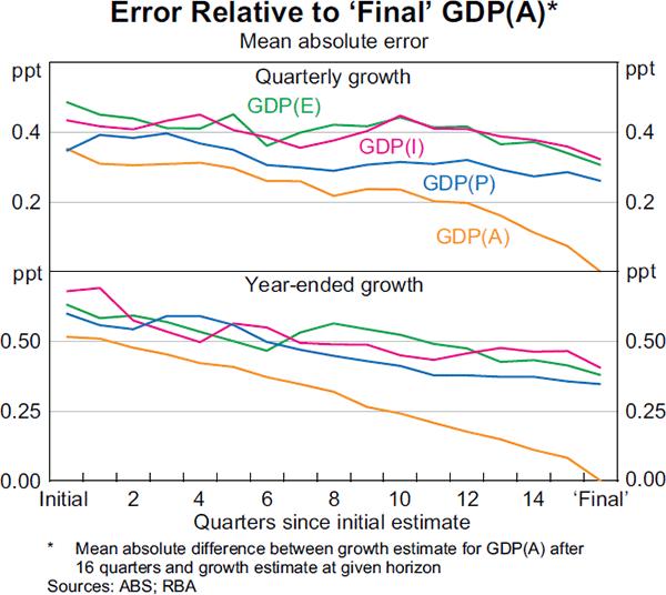
While reliability is one useful metric for judging the quality of early GDP growth estimates, it does not indicate which measures are more accurate in real time, in terms of their closeness to the ‘final’ estimate of growth in GDP(A).[3] Graph 2 shows the mean absolute error of each measure of GDP compared with final GDP(A).[4] Both in quarterly and year-ended terms, initial estimates of GDP(P) have tended to be closer to that of final GDP(A) than either GDP(E) or GDP(I). On a quarterly basis, initial estimates of GDP(P) have been as close as initial estimates of GDP(A), suggesting that initial estimates of GDP(P) have, on average, provided a real-time read on ‘final’ GDP growth as accurate as the ABS's preferred measure (although this is not the case for initial estimates of year-ended growth). On the other hand, initial estimates of GDP(E) and GDP(I) have been somewhat less accurate predictors of ‘final’ GDP(A), on both a quarterly and year-ended basis.
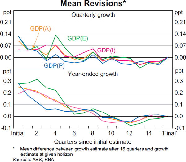
Another gauge of the quality of real-time estimates is whether they tend to overstate or understate ‘final’ estimates, that is, whether they are biased. A simple average of revisions at each horizon is shown in Graph 3. The first estimate of quarterly GDP(A) growth has tended to be revised upwards by around 0.1 percentage points, although the mean revision falls close to zero relatively quickly.[5] In year-ended terms, initial estimates have been revised upwards by 0.2 percentage points on average. Early estimates have tended to be revised up for each of the three GDP measures, although the mean revision for GDP(P) approaches zero quite quickly. GDP(E) generally had a relatively large (positive) mean revision until around the fifth estimate in year-ended terms. Revisions to a given quarter through time have tended to be negatively correlated, suggesting that if GDP growth for a particular quarter was revised up in one release of the data, it was more likely to be revised down in the next release (although the negative correlations were typically small).
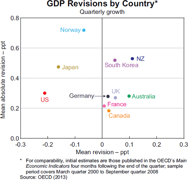
While the revisions to Australian GDP, including the average upward revision to initial GDP growth estimates, have been non-trivial in size, they have been consistent with international experience (Graph 4). The mean absolute size of revisions in Australia has been similar to that for a number of large advanced economies, and smaller than that for some smaller economies.[6] The mean revision to initial estimates in Australia has been somewhat larger than in some other economies, though in line with New Zealand and smaller in absolute size than in the United States and Japan.
Revisions around Turning Points
The effectiveness of macroeconomic policy in part relates to the ability of policymakers to respond quickly to changing economic conditions. It is important, therefore, to consider how measures of GDP growth are revised around turning points in the economy. Because initial GDP growth estimates are produced without all the information that will eventually become available, business cycle turning points may not be fully apparent in real time. For example, during a downturn estimates of GDP growth may be initially overstated if it takes time for the ABS to be informed of business closures. For this reason, one could expect downward revisions to growth during a downturn and upward revisions to growth during an upswing.
The dates of peaks and troughs in the business cycle can be estimated using growth in GDP(A) and a Bry-Boschan algorithm.[7] This method identifies five peaks and four troughs in the business cycle between 1991 and 2012; Table 2 presents the average size of revisions around these peaks and troughs.[8] GDP(I) and GDP(E) growth estimates have indeed tended to be revised down following peaks in the cycle, while all GDP measures have tended to be revised up following troughs in the cycle during the past 20 years. More striking perhaps is the fact that peaks and troughs have typically been much less apparent in real time. Revisions to GDP(P) have been relatively more stable around turning points than revisions to the other measures of GDP.
| Peaks(b) | Troughs(c) | |||||
|---|---|---|---|---|---|---|
| Two prior quarters | Peak | Two subsequent quarters | Two prior quarters | Trough | Two subsequent quarters | |
| GDP(A) | 0.13 | 0.67 | 0.01 | 0.17 | −0.36 | 0.22 |
| GDP(E) | 0.17 | 0.96 | −0.07 | 0.22 | −0.86 | 0.24 |
| GDP(I) | 0.12 | 0.75 | −0.00 | 0.18 | −0.28 | 0.20 |
| GDP(P) | 0.12 | 0.31 | 0.11 | 0.12 | 0.07 | 0.21 |
|
(a) Business cycle dated by running a quarterly Bry-Boschan algorithm over the latest
estimates of GDP growth for the period 1991–2008 Sources: ABS; RBA |
||||||
One challenge when conducting analysis only around turning points is that the business
cycle tends to move slowly, and so the sample of peaks and troughs is limited.
One way to take advantage of the full sample of revisions when assessing the
relationship between revisions and the business cycle is to look at the correlation
between revisions to GDP growth  and an ‘acceleration factor’
  , which captures the
speed at which the economy is expanding (similar to Dynan and Elmendorf 2001).
A positive correlation suggests that there is a tendency for revisions to
become more positive when the economy is speeding up and less
positive (or even negative) when the economy is slowing down. The results
support the proposition that the pattern of revisions to GDP has been related
to the business cycle, with correlations of 0.24 for GDP(P), 0.54 for GDP(I)
and 0.72 for GDP(E). The relatively low correlation for GDP(P) is consistent
with the finding above that revisions to GDP(P) have been less affected by
business cycle turning points.
Revisions to GDP Components
To further explain the patterns in revisions to GDP growth, the size and direction of revisions to the underlying components of GDP can be examined. An analysis of revisions at the component level is also important in its own right, given that policymakers examine GDP components to understand the economy more deeply. For example, the household saving ratio – which is the residual of household consumption and household disposable income, expressed as a share of income – is typically used as an indicator of households' propensity to spend.
Size of revisions
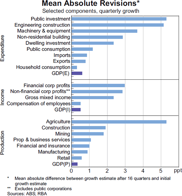
An analysis of mean absolute revisions to quarterly growth indicates that revisions to the components have tended to be larger than the revisions to GDP itself (Graph 5).[9] This is because GDP is inherently ‘smoother’ than its components (see below) as the growth rate of its various components is not perfectly correlated and some of the measurement errors in the GDP components offset each other when they are aggregated. Some revisions also involve a reallocation of growth between components. The size of revisions varies substantially; for expenditure components, revisions to quarterly growth ranged from 0.3 percentage points for household consumption, to more than 5 percentage points for public investment and engineering construction.
However, the substantial variation in the size of revisions between the components of GDP needs to be viewed in the context of the relative volatility of each series. A volatile series, such as public investment, is much more likely to be subject to larger percentage point revisions on average than a smoother series, such as household consumption. The data show that indeed there has been a strong positive relationship between the absolute size of revisions and the volatility of growth in the components of GDP (Graph 6).
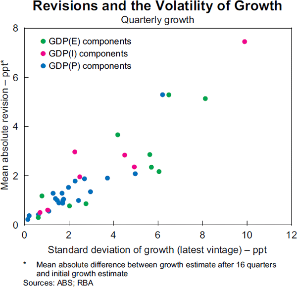
Once adjustments are made to account for differences in the volatilities of the components, public consumption is the component of GDP(E) with the largest revisions. The ‘signal’ provided by these data in real time has often been obscured by ‘noise’, which is consistent with the ABS's own assessment that initial estimates of public consumption have been a ‘relatively poor indicator of later estimates’ (ABS 2007, p 63).
Main drivers of GDP revisions
To estimate which components make the largest contribution to GDP revisions, the mean absolute revision statistics for each component are weighted by their shares of nominal GDP. This takes into account the fact that a 1 percentage point revision to household consumption results in a much larger revision to GDP than a 1 percentage point revision to public investment, owing to the larger share of household consumption in GDP. This method of weighting revisions by GDP shares – which is similar to calculating revisions to contributions to real GDP growth – also allows the relative importance of revisions to the change in inventories to be estimated, for which meaningful growth rates could not otherwise be calculated.[10]
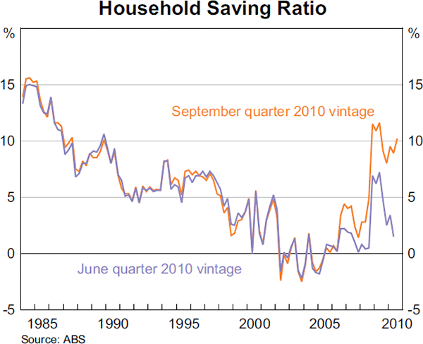
The largest contributor to GDP revisions on the expenditure side of the accounts has been the change in inventories (Graph 7). This is an extremely volatile series that is calculated as the difference between estimates of opening and closing inventory levels in each quarter, and it is very difficult to measure accurately (ABS 2007). Other major contributors to GDP(E) revisions include public consumption and public investment. Revisions to household consumption have typically played a smaller role in GDP(E) revisions, despite its large weight in GDP. Nevertheless, revisions to consumption have still had important implications for macroeconomic assessments; in late 2010, the ABS revised the estimates of household saving, which reflected both a downward revision to consumption and an upward revision to household income. This revision lifted estimated household saving by $45 billion in 2009/10, or about 5½ per cent of income, which suggested that households had changed their saving propensity by more than earlier thought (Graph 8).
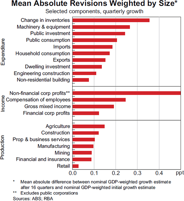
The largest contributor to revisions to growth in GDP(I) has been private non-financial corporate profits, reflecting the series' large propensity for revision and sizeable share of GDP. In contrast, on the production side of the accounts no particular component stands out as having been a significant driver of overall GDP(P) revisions.
It is important to note, however, that revisions to GDP components in any given quarter will be offsetting to some degree, thereby mitigating the overall revision to GDP growth. For example, an upward revision to imports in a quarter may be matched, in both an accounting and conceptual sense, by corresponding upward revisions to other expenditure components such as household consumption.
Direction of revisions
The source of the average positive revision to early estimates of GDP can be better understood by examining the mean revisions to each of the GDP components (Graph 9). The upward revisions to early estimates of GDP growth over the period from 1998 to 2008 reflected upward revisions to most GDP components: for the 39 components analysed across the three measures of GDP, 29 tended to be revised higher over time. However, this tendency was only statistically significant at the 10 per cent level for three of the components (engineering investment, construction gross value added and financial corporations' profits).
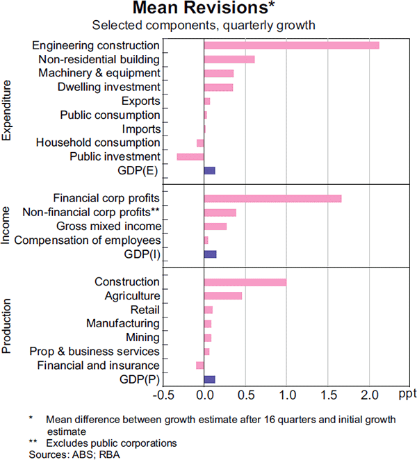
On the expenditure side, early estimates of the investment components have been particularly prone to subsequent upward revision over our sample period at least. First estimates of engineering investment growth were revised up by 2.1 percentage points on average. Residential and non-residential building construction estimates have also tended to be revised up over time, partly owing to upward revisions to building approvals flowing through to higher investment.[11] On average, the tendency for the investment components to be revised upwards typically dissipated after around one to two quarters, with the exception of machinery & equipment investment, with real-time estimates having tended to understate ‘final’ values for several years.
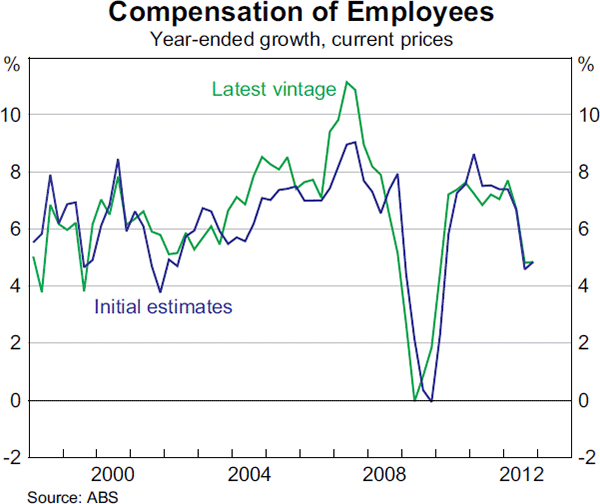
On the income side, along with corporate profits, gross mixed income and compensation of employees have also tended to be understated in real time. Initial estimates of compensation of employees noticeably understated growth between the mid 2000s and late 2007 (Graph 10), and indicated a smaller pick-up in labour costs than in the latest vintage. Such data revisions can complicate the assessment of inflation pressures in the economy. Since the income components are published on a nominal (value) basis rather than on a real (volume) basis, these revisions can also be a result of upward revisions to prices. Consistent with this, nominal GDP has tended to experience larger upward revisions on average than real GDP, reflecting upward revisions to the GDP deflator.
Implications
The above analysis illustrates that real-time estimates of GDP growth are subject to significant revisions, so users should be careful not to over-interpret quarterly changes based on early vintages of data. It also highlights the importance of gathering and monitoring a wide range of other timely data and information.
Over the sample used in this article, early estimates of GDP growth tended to understate ‘final’ GDP growth to some degree. In principle, users can take this into account when considering the latest GDP data, but it is not clear that such a tendency will persist in the future. In particular, methodological improvements may reduce this tendency over time. The observed positive average revisions to early estimates may also have been driven by the nature of shocks affecting the economy during the sample period, which may not be repeated in coming years. For example, the impact of the sharp increase in the terms of trade on activity and profits may not have been fully apparent until the receipt of detailed tax data, which are only available with some delay. To the extent that the direction of revisions is somewhat related to the economic cycle, it is also relevant that the sample predominantly covers a period of relatively strong growth without any significant downturns.
Considering the different measures of GDP, when judged on the various metrics in this article, real-time estimates of GDP(P) performed almost as well as the real-time estimates of GDP(A) and better than the real-time estimates of GDP(E) and GDP(I).[12] Accordingly, for early GDP estimates, there seems to be some merit in placing relatively more weight on the early estimates of GDP(P).[13] However, once again, historical patterns may not necessarily persist in the future.
Given the extent of revisions to early estimates, it would be useful if data users could explicitly predict revisions in order to improve real-time estimates. In principle, this would be possible as subsequent data are published that either feed directly into the measurement of GDP or are correlated with revisions. Given that initial GDP estimates in Australia incorporate most of the regularly available monthly and quarterly data for the given quarter, this approach seems less likely to be fruitful than in countries in which preliminary or ‘flash’ GDP estimates are published using data for only the first two months of the quarter (such as in the United States), which can then be revised by users as the final month's data are subsequently published.[14]
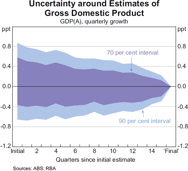
Another approach is to consider the distribution of likely ‘final’ values by constructing confidence intervals around the early estimates of GDP.[15] Confidence intervals can be constructed using the historical root mean squared error of past estimates compared with ‘final’ estimates (and assuming errors are normally distributed), with an adjustment also being made for the tendency for estimates to be initially understated. This approach is illustrated in Graph 11, and suggests that, based on past experience, the ‘final’ estimate of GDP(A) growth in any given quarter can be as much as 0.8 percentage points away from early estimates, with a 90 per cent confidence level. This serves to highlight the considerable uncertainty around published GDP estimates in real time.
Conclusion
Policymakers not only face uncertainty about the future, but also about the present and the past, since real-time data are subject to revision. This article illustrates the pattern and size of revisions to Australian GDP growth and its underlying components over the past decade or so. Revisions to early estimates of GDP growth have tended to be sizeable and in an upwards direction, though these characteristics are not unusual by international standards. Of the three measures of GDP growth, the production measure has performed as well, or better, than the other measures as a real-time indicator of the ‘final’ GDP growth estimate. Policymakers and other users of GDP data could attempt to anticipate revisions or use devices such as confidence intervals to illustrate the uncertainty around the data. The uncertainty also highlights the importance of gathering and monitoring a wide range of data and information when assessing current economic conditions.
Appendix A
| Share of GDP in 2011/12(a) Per cent | Mean absolute revision Percentage points | Mean absolute revision weighted by size(b) Percentage points | Mean revision Percentage points | |
|---|---|---|---|---|
| Household consumption | 54 | 0.3 | 0.2 | −0.1 |
| Dwelling investment | 5 | 2.3 | 0.1 | 0.3 |
| Machinery & equipment | 6 | 3.7 | 0.3 | 0.4 |
| Non-residential building | 3 | 2.9 | 0.1 | 0.6 |
| Engineering construction | 6 | 5.1 | 0.1 | 2.1 |
| Public consumption | 18 | 1.2 | 0.2 | 0.0 |
| Public investment | 5 | 5.3 | 0.2 | −0.3 |
| Exports | 21 | 0.8 | 0.2 | 0.1 |
| Imports | 21 | 0.9 | 0.2 | 0.0 |
| Change in inventories(c) | na | na | 0.4 | na |
| GDP(E) | 100 | 0.6 | 0.6 | 0.1 |
| Compensation of employees | 48 | 0.5 | 0.2 | 0.0 |
| Non-financial corp profits (private) | 20 | 2.8 | 0.5 | 0.4 |
| Non-financial corp profits (public) | 1 | 7.5 | 0.2 | −1.2 |
| Financial corp profits | 5 | 3.0 | 0.1 | 1.7 |
| General government GOS(d) | 2 | 0.4 | 0.0 | 0.1 |
| Dwellings GOS(d) | 7 | 0.6 | 0.0 | 0.1 |
| Gross mixed income | 8 | 2.4 | 0.2 | 0.3 |
| GDP(I) | 100 | 0.5 | 0.5 | 0.0 |
| Agriculture | 2 | 5.3 | 0.1 | 0.5 |
| Mining | 10 | 1.8 | 0.1 | 0.1 |
| Manufacturing | 7 | 0.9 | 0.1 | 0.1 |
| Utilities | 2 | 1.0 | 0.0 | 0.1 |
| Construction | 7 | 1.9 | 0.1 | 1.0 |
| Wholesale | 4 | 1.0 | 0.0 | −0.2 |
| Retail | 4 | 0.6 | 0.0 | 0.1 |
| Accommodation & food | 2 | 1.3 | 0.0 | 0.1 |
| Transport | 5 | 1.0 | 0.0 | 0.3 |
| Media & telecommunications | 3 | 1.5 | 0.1 | 0.0 |
| Financial & insurance services | 10 | 1.0 | 0.1 | −0.1 |
| Property & business services(e) | 11 | 1.1 | 0.1 | 0.1 |
| Public administration | 5 | 1.3 | 0.1 | 0.3 |
| Education | 4 | 0.4 | 0.0 | 0.2 |
| Health | 6 | 1.3 | 0.1 | 0.4 |
| Arts & recreation | 1 | 2.1 | 0.0 | 0.2 |
| Other services | 2 | 1.9 | 0.0 | −0.2 |
| Ownership of dwellings | 8 | 0.2 | 0.0 | 0.0 |
| GDP(P) | 100 | 0.3 | 0.3 | 0.1 |
| Memo: | ||||
| Nominal GDP | 100 | 0.5 | 0.5 | 0.2 |
| GDP implicit price deflator | na | 0.4 | na | 0.1 |
|
(a) The shares of GDP(E) do not sum to 100 per cent due to the exclusion of several
smaller investment components; the shares of
GDP(I) and
GDP(P) do not sum to 100 per cent due to the exclusion of taxes
less subsidies Sources: ABS; RBA |
||||
Footnotes
The authors are from Economic Group. [*]
GDP(E) is calculated as the sum of all expenditures by households, businesses and governments on final production, plus exports and the change in inventories, less imported goods and services. GDP(I) measures the income received for providing labour and capital services as inputs to production. GDP(P) measures the value of production in the economy as the difference between the value of outputs and the value of intermediate inputs consumed in production. Conceptually, the three measures should be equal, but in practice the measures differ because they are constructed from different data sources and have varying degrees of measurement error. For more detail on the ABS's data construction methods, see ABS (2007, 2011, 2012). The ABS is one of only a few statistical agencies in the world to compile and publish all three measures of GDP. [1]
For a comprehensive review of the literature on revisions to macroeconomic data, see Croushore (2011). [2]
A GDP figure that is never revised would not, in practice, indicate high quality. [3]
While the annual reconciliation process conducted by the ABS equalises the GDP measures in annual terms (for financial years prior to the latest complete year), discrepancies typically remain between the measures on a quarterly basis. [4]
The mean revision for the first estimate of GDP(A) growth is statistically different from zero at the 10 per cent significance level, using standard errors which are robust to heteroscedasticity and autocorrelation. The results may be somewhat dependent on the sample (September quarter 1998 to December quarter 2008), which spans a period of relatively strong economic growth. [5]
A measure of absolute revision that adjusts for the difference in average rates of economic growth across countries shows a broadly similar pattern, albeit with Germany, France, Japan and the US recording relatively larger mean absolute revisions. [6]
Because peaks and troughs can move across vintages, in this section ‘final’ GDP is defined as the latest published vintage. For an example of the use of the quarterly Bry-Boschan algorithm to date cycles in economic data, see Harding and Pagan (2002). [7]
Troughs and peaks prior to 1991 are excluded because the four measures of GDP were not concurrently published before that time. [8]
Graphs 5, 7 and 9 exclude several components of GDP. The statistics for a larger group of components of GDP are listed in Table A1. The components of GDP(I) are in nominal terms. [9]
Since the change in inventories can take positive or negative values, the growth rate of the change in inventories can become arbitrarily large in magnitude, or vary perversely in sign, if stocks cease being accumulated or actually decline. For this reason, in Graph 7 the mean absolute contribution of the change in inventories to GDP growth is calculated directly. [10]
Revisions to building approvals data flow through to the data for residential and non-residential building investment in the national accounts because the sample frame that is used for the ABS Building Activity Survey (which provides the quarterly indicators for the national accounts components) is based on building approvals details. Using monthly data over the period 2006–2012, initial estimates of the number of residential building approvals were revised up by 5 per cent on average, while the value of non-residential building approvals were revised up by 10 per cent on average. [11]
In a similar vein, Nalewaik (2010, 2011) suggests that in the United States GDP(I) may be a better measure of GDP than the more commonly used GDP(E). Auroba et al (2011) also argue that in the United States, GDP(I) and GDP(E) should be combined to produce a better measure of GDP (akin to GDP(A) in Australia). [12]
As each of the three measures has an equal weight in GDP(A), this raises the question of whether a different weighting scheme for early estimates might provide a more accurate estimate of ‘final’ GDP(A). One approach is to estimate a regression of ‘final’ GDP(A) growth on the initial GDP growth estimates for each of the three measures, which suggests a weighting scheme of 0.5 for GDP(P), 0.4 for GDP(I) and 0.1 for GDP(E) (where the coefficients are constrained to sum to 1). However, this alternative measure of GDP did not outperform the initial estimate of GDP(A) as an indicator of ‘final’ GDP(A) over the 1998–2008 sample period. [13]
It might be possible to predict revisions to some degree using a broad range of timely economic indicators (on the basis that such indicators may contain information not yet captured by the available data underpinning the national accounts); however, such predictions would rely on relationships that may not necessarily hold in the future. [14]
This approach is employed by the Bank of England, which uses state-space modelling techniques to construct confidence intervals that are routinely presented as fan charts in its quarterly Inflation Report. [15]
References
ABS (Australian Bureau of Statistics) (2007), ‘Quality Dimensions of the Australian National Accounts’, ABS Cat No 5216.0.55.002.
ABS (2011), ‘Spotlight on National Accounts: Which is the Best Short-term Measure of Gross Domestic Product?’, ABS Cat No 5202.0, May.
ABS (2012), ‘Australian System of National Accounts: Concepts Sources and Methods’, ABS Cat No 5216.0, edn 3.
Aspden C (1990), ‘Which is the Best Short-term Measure of Gross Domestic Product? A Statistical Analysis of the Short-term Movements of the Three Measures of Gross Domestic Product and their Average’, ABS Cat No 5206.0, June.
Auroba B, F Diebold, J Nalewaik, F Schorfheide and D Song (2011), ‘Improving GDP Measurement: A Forecast Combination Perspective’, NBER Working Paper No 17421.
Croushore D (2011), ‘Frontiers of Real-time Data Analysis’, Journal of Economic Literature, 49(1), pp 72–100.
Dynan K and D Elmendorf (2001), ‘Do Provisional Estimates of Output Miss Economic Turning Points?’, Federal Reserve Board Working Paper No 2001/52.
Harding D and A Pagan (2002), ‘Dissecting the Cycle: A Methodological Investigation’, Journal of Monetary Economics, 49(2), pp 365–381.
Nalewaik J (2010), ‘The Income- and Expenditure-Side Estimates of US Output Growth’, Brookings Papers on Economic Activity, Spring, pp 71–106.
Nalewaik J (2011), ‘The Income- and Expenditure-Side Estimates of US Output Growth: An Update to 2011Q2’, Brookings Papers on Economic Activity, Fall, pp 385–403.
OECD (Organisation for Economic Co-operation and Development) (2013), ‘Main Economic Indicators: Original Release Data and Revisions Database’, accessed 1 February 2013. Available at <http://stats.oecd.org/mei/default.asp?rev=1&lang=e>.