Bulletin – September 2015 Payments The Life of Australian Banknotes
- Download the article 285KB
Abstract
An assessment of the likely life of a banknote is an important input to a currency issuer's planning. Without accurate predictions of banknote life, there is the potential to incur the economic costs of producing and storing excess banknotes or, conversely, in an extreme case, of not being able to meet the public's demand. The life of a banknote, however, is not directly observed and must be estimated. This article discusses some traditional measures of banknote life and provides some alternative estimates using ‘survival’ modelling.
Introduction
To make decisions on banknote production, processing, distribution and storage requirements, it is important for currency issuers to understand how long banknotes typically remain in circulation before they need to be replaced with new banknotes.
This article examines three ways of estimating the life of banknotes using data commonly available to currency issuers on the number of banknotes circulating, destroyed and issued for the first time. Two of the methods are based on turnover, and are often used due to their ease of calculation and simple data requirements. The third method is based on more complex statistical models that predict the probability of banknotes surviving over time. The results from these methods can also be compared with samples of banknotes collected from circulation. More detailed analysis and further technical information on the construction of the three estimation methods are available in a more extensive research paper (see Rush (2015)).
The Life Cycle of Banknotes
To examine the life of a banknote, it is important to understand the manner in which banknotes are issued and circulated. Banknotes are produced and then stored until required to meet public demand (Figure 1). Once issued, they may spend time being held as a store of value or in active circulation (being used in transactions). In Australia, banknote demand generally grows in line with nominal GDP and shows seasonal peaks each year, particularly during Easter and December. Following these seasonal peaks, banknotes in excess of the public's requirements (‘surplus fit’ banknotes) are returned to the Reserve Bank via the commercial cash industry to be reissued at a later date.
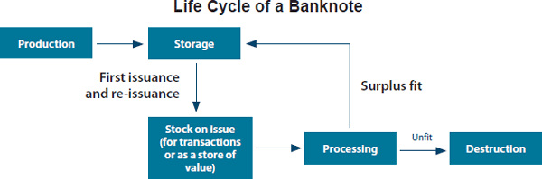
As a result of being used in circulation, banknotes deteriorate in quality and eventually become unfit. Banknotes may become unfit due to randomly occurring mechanical defects (including staple holes and tears) or gradually through the process of ink wearing off as the banknote is handled. The length of time before becoming unfit can differ considerably from banknote to banknote – one used repeatedly in transactions will become unfit sooner than one stored in a protected location.
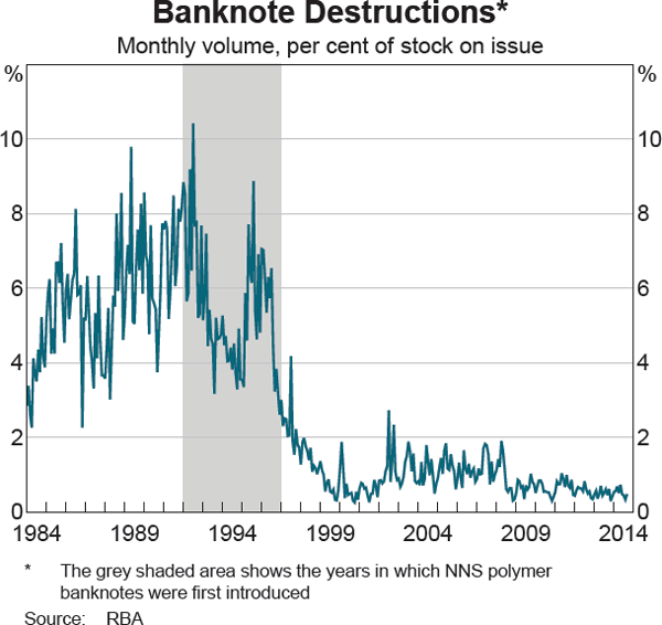
Banknotes returned to the Bank via the commercial cash system are assessed and validated. Fit banknotes are eventually reissued into circulation and unfit banknotes are destroyed.[1] Banknote destructions fluctuate considerably from month to month, but the average rate of destruction of banknotes in circulation fell from 5.7 per cent per month prior to 1992 to 1.0 per cent per month after the introduction of the more durable polymer New Note Series (NNS) banknotes (Graph 1).
Estimating the Life of Banknotes
Ideally, the life of every banknote could be studied by recording the dates when they were first issued into circulation and when returned for destruction. While this option is becoming increasingly available to currency issuers, it cannot be applied to the large stock of banknotes already in circulation. Instead, banknote life can be estimated using a number of different methods that make use of aggregate data on the number of banknotes circulating, destroyed and issued for the first time.
Traditional steady-state or turnover method
Currency issuers commonly use a simple steady-state[2] or turnover formula to estimate the average life of a banknote (over any given 12-month period), calculated as:

The median banknote life can be calculated by finding the point at which 50 per cent of banknotes survive, using the assumption that the probability that a banknote becomes unfit at a given point in time is given by the inverse of the estimated average life. This assumes that the probability of a banknote becoming unfit is invariant to the time it spends in circulation.[3] However, since some banknotes last a very long time (e.g. those kept in safe locations as a store of value), the estimate of average banknote life will be larger than the median estimate.
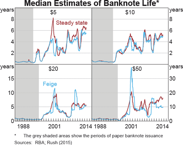
Using this method for Australia's $5 to $50 denominations, a number of observations can be made:
- As expected, the median life is lower than the average life for all denominations and time periods (Graphs 2 and 3).
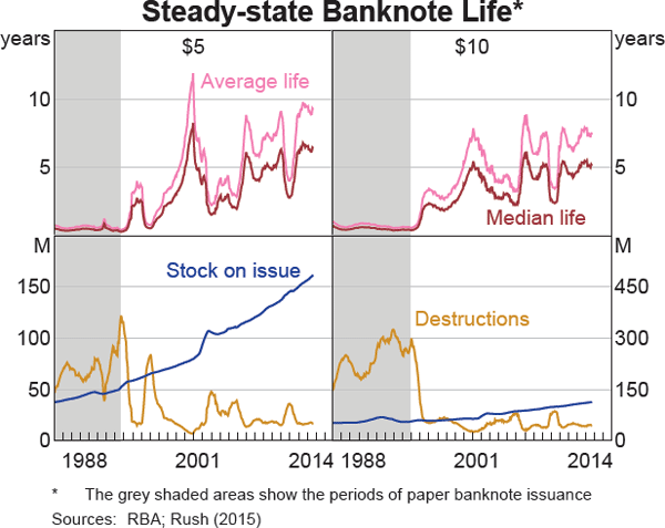
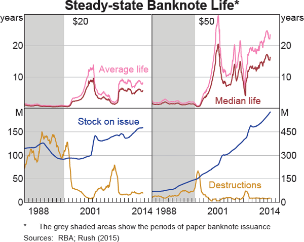
- Since the issuance of NNS polymer banknotes, the median life has ranged widely across denominations – from 3.5 years for $5 banknotes up to 10 years for $50 banknotes – even though all Australian banknote denominations are produced with the same technology and have identical security features.[4] This result is expected since lower-value denominations are more likely to be used in transactions, whereas higher-value denominations are more likely to be used as a store of value.
- For all denominations, the life of polymer banknotes is longer than the equivalent paper banknotes (which had median life spans ranging from around six months to 1.5 years for the $5 and $50 denominations respectively). The volatility of the estimates also increased after the introduction of polymer banknotes as their life became progressively greater than the 12-month period included in the formula.[5]
‘Feige’ steady-state method
A limitation of the steady-state formula discussed above is that it is biased by growth in the number of circulating banknotes. This bias arises because destructions (the denominator) tend to reflect banknotes that were issued some time ago, whereas the number of banknotes in circulation (the numerator) includes banknotes that have only recently been issued. In other words, the average age of banknotes on issue falls if the population of banknotes is growing due to the addition of new banknotes. Feige (1989) derives an alternative formula for average banknote life that aims to reduce this bias by adjusting the denominator by the number of banknotes issued into circulation for the first time.
As expected, using the Feige method results in banknote life estimates that are generally a little lower than the traditional steady-state results (Graph 4). The results of the Feige equation appear to be less volatile over time for the paper series and the low-value $5 and $10 polymer banknotes, whereas for the $20 and $50 polymer banknotes there are still some significant fluctuations. This is most likely due to the fact that the Feige equation only adjusts for new banknotes when they are first issued into circulation, but does not satisfactorily control for situations where banknotes are issued and then temporarily withdrawn from circulation. For example, in the lead-up to January 2000, large volumes of new banknotes were issued to meet precautionary demand (owing to concerns about Y2K problems). These extra banknotes were withdrawn when no longer required and reissued later. As a result, there was a sharp decline in the estimated banknote life in 1999 and a sharp increase a year later.
Limitations of the steady-state methods
While easy to understand and simple to calculate, the traditional and Feige steady-state methods have a number of limitations:
- The steady-state measures do not provide much information about how the probability of becoming unfit varies over a banknote's lifetime or how life spans vary within a banknote denomination. It is possible that the probability of a banknote becoming unfit could increase over time due to inkwear. The life span of banknotes is also likely to vary, even within a denomination, since not all banknotes are treated in the same way by the public. For example, banknotes used as a store of value are likely to stay in good condition (and thus, should have a longer life) compared with banknotes used repeatedly in transactions.
- The steady-state methods cannot control for changes to currency issuer policies, including the issuance of a new banknote series or measures taken to improve the quality of banknotes in circulation. For example, from time to time the Bank conducts targeted quality programs (known as cleansing programs), which involve accelerating the withdrawal of a specific denomination in circulation and replacing any unfit banknotes with new banknotes. During these cleansing programs, banknote life (as estimated by the steady-state measures) initially declines since destructions are high compared with the stock of banknotes on issue. Their typical life subsequently becomes longer since the remaining stock of banknotes on issue is of a higher quality and fewer banknotes become unfit for a time.
- Fluctuations in banknote demand can also cause volatility in the two steady-state measures. For example, in late 2008, the demand for $50 banknotes increased sharply in response to concerns associated with the global financial crisis (GFC). Although those concerns quickly abated, it took more than two years to unwind the excess supply of $50 banknotes in circulation. The sharp increase in circulating $50 banknotes was not mirrored by large increases in destructions (since $50 banknotes tend to last many years) and thus, the banknote life estimated by the turnover formulas increased and remained at higher levels for several years.
Survival modelling
More complex models of the survival of banknotes can be estimated to address some of the limitations of the two steady-state methods. These models estimate banknotes' probability of survival, and the number of banknotes from each issuance date that survive over time, in order to reconcile the total number of fit banknotes observed each month.[6] Unlike the simple turnover formulas, these survival models do not assume a constant probability of a banknote becoming unfit and can also take into account the fact that some banknotes are used as a store of value, or for numismatic purposes (i.e. study or collection), and are unlikely to become unfit. The survival models suggest that these stored or numismatic banknotes represent around 30 per cent of $50 banknotes and 10–15 per cent of the lower-value $5, $10 and $20 banknotes. In addition, the survival models include other variables to take into account factors that affect the supply of and demand for banknotes. For example, they can take into account the greater demand for $50 banknotes around the onset of the GFC and indicate that the probability of survival declined a little over the period, which suggests that banknotes were handled more frequently during the crisis.
The median estimates of banknote life resulting from the survival models are far more stable over time than the results of the steady-state methods (Graph 5). This makes the estimates of the survival models more useful for long-term decision-making, where the currency issuer needs to abstract from the fluctuations in banknote life estimates caused by one-off events. The disadvantage of the survival models relative to the steady-state methods is that they require longer time series of data before estimates can be produced.
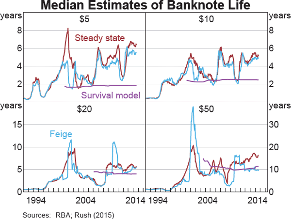
Reassuringly, averaged over long spans of time, the median banknote life spans are quite similar across all three methods and are most similar for the $50 denomination (Table 1). All three methods predict longer life spans as the denomination value increases, though the difference between the median life of the lowest- and highest-value denominations is largest under the survival models' estimates.
Back-testing the Models
The article has so far focused on the expected average or median life span of a newly issued banknote predicted by three estimation methods. The methods can also be used to estimate the median age of banknotes in circulation or destroyed at a point in time, which can be validated against the age of banknotes observed in two sampling programs conducted by the Bank.
| Denomination | Steady state | Feige | Survival models |
|---|---|---|---|
| $5 | 3.5 | 3.0 | 1.9 |
| $10 | 3.5 | 3.2 | 2.5 |
| $20 | 4.1 | 3.9 | 4.0 |
| $50 | 10.0 | 8.9 | 10.7 |
|
Sources: RBA; Rush (2015) |
|||
In Australia, unfit banknotes are returned to the National Note Processing and Distribution Centre (NNPDC) where they are validated, assessed and destroyed. A sample of around 800,000 unfit banknotes was extracted in 2011 and sorted into production vintages based on the unique serial number printed on each banknote.[7] The median age estimates derived from the steady-state method are higher than those in the sample of unfit banknotes, particularly for $10 banknotes (Table 2). The results are most similar between the steady-state method and the sample for $5 banknotes; however, the 2011 period coincided with a cleansing program for the $5 which, as discussed previously, caused the steady-state method to have lower life predictions than would otherwise have been the case. The median estimates for the age of unfit banknotes generated by the survival models are lower than the steady-state estimates and, on average, are closer to the results of the sample.
The Bank also conducts a Commercial Cash Sampling (CCS) program, which collects unsorted banknotes from cash-in-transit companies across Australia. The purpose of this program is to assess the quality of circulating banknotes, but it can also be used to examine the distribution of ages of banknotes that actively circulate. For three sample periods (February in each of 2011, 2012 and 2013), the traditional steady-state method generally implies higher median ages for banknotes on issue than predicted by the survival models and the CCS sample methodology (Table 3). The median ages of banknotes in circulation from the CCS samples tend to be closer to those predicted by the survival models.
| Denomination | Traditional steady state | Survival models | Unfit sample |
|---|---|---|---|
| $5 | 5.3 | 4.3 | 5.2 |
| $10 | 7.3 | 4.4 | 4.9 |
| $20 | 5.3 | 4.4 | 4.6 |
| $50 | 6.6 | 5.4 | 6.1 |
|
Sources: RBA; Rush (2015) |
|||
| Denomination | Traditional steady state | Survival models | Unfit sample | ||||||
|---|---|---|---|---|---|---|---|---|---|
| 2011 | 2012 | 2013 | 2011 | 2012 | 2013 | 2011 | 2012 | 2013 | |
| $5 | 5.7 | 5.9 | 6.8 | 5.5 | 6.0 | 6.7 | 4.8 | 5.2 | 5.9 |
| $10 | 4.8 | 5.9 | 7.2 | 4.6 | 5.3 | 6.6 | 4.4 | 5.0 | 6.6 |
| $20 | 5.4 | 5.9 | 6.4 | 5.3 | 5.9 | 6.3 | 4.3 | 5.0 | 5.7 |
| $50 | 6.7 | 7.2 | 7.8 | 5.5 | 6.1 | 6.5 | 5.1 | 5.6 | 6.1 |
|
Sources: RBA; Rush (2015) |
|||||||||
Conclusions
The median life of Australian banknotes spans a wide range across denominations – from around 2–3 years for the $5 up to around 10 years for the $50 – with little variation across the methods of calculation over the long run. The two steady-state methods are easy to calculate, and indicate that polymer banknotes last considerably longer than the equivalent paper denominations. These methods are, however, unable to account for supply and demand shocks and the estimates have considerable volatility from month to month. The survival models correct for some of the limitations of the steady-state methods and produce more stable and intuitive estimates of banknote life. They are able to provide other useful information, such as the proportion of banknotes for each denomination that actively circulate (as opposed to being used for store of value or numismatic purposes). The survival models' predictions for banknote survival are also, on average, more consistent with samples of circulating and unfit banknotes. Given the advantages of the new survival models, they will be a useful complement to the traditional estimation methods and can help the Bank's long-term decision-making.
Footnotes
The author is from Economic Analysis Department but the majority of this work was completed in Note Issue Department. [*]
For more information on the Bank's damaged banknote policy and sorting standards see <http://banknotes.rba.gov.au/damaged-banknotes/damaged-banknotes-policy/>. [1]
It is often known as the ‘steady-state’ method since it was thought that after a banknote series had been circulating for a number of years, the growth in banknote destructions and circulation would stabilise and the estimate of banknote life would become relatively constant. [2]
See Rush (2015) for more details. [3]
Since $100 banknotes are generally held by the public as a store of value, they do not tend to actively circulate and with such little handling do not deteriorate significantly over time. Indeed, less than 10 per cent of $100 polymer banknotes ever issued have been returned to the RBA as unfit banknotes, making estimates of $100 banknote life uninformative. [4]
When the life of banknotes had been less than a year, comparing the number of unfit banknotes observed in a year relative to the stock on issue over the same year would have given a reasonable estimate of the average or median life span. As the life increases beyond a year, however, the formula may not always give an accurate estimate, particularly around periods when a lot of banknotes are issued or old banknotes are destroyed. (For example, if many old banknotes happened to be destroyed in a particular year, the life span estimates for that year are likely to be underestimated. The remaining stock of banknotes on issue would be much younger and, therefore, unlikely to become unfit for a time and so subsequent life estimates are likely to be overestimated for some time.) [5]
Further technical information and details on these non-linear regression models are available in the research paper on the life of Australian banknotes, see Rush (2015). [6]
The first two numbers of a banknote's serial number identify the year a banknote was manufactured; for more information, see <http://banknotes.rba.gov.au/production-and-distribution/production/>. [7]
References
Feige EL (1989), ‘Currency Velocity and Cash Payments in the U.S. Economy: The Currency Enigma’, MPRA Paper No 13807 .
Rush A (2015), ‘The Life of Australian Banknotes’, RBA Research Discussion Paper No 2015-10.