RBA Annual Conference – 1993 The Role of the Exchange Rate in Monetary Policy – the Experience of Other Countries Michael Artis
1. Introduction
In the past 15 years we have seen two significant episodes of exchange rate targeting, each very different in character and in their proximate objectives. One is the phase of exchange rate targeting inaugurated by the Plaza Accord in September 1985; the other is the system of exchange rate targeting inaugurated by the establishment of the European Monetary System (EMS) in 1979.
The former had as its proximate objective the correction of a substantial misalignment – that is, it had a real exchange rate or competitiveness objective. A decline in the nominal US dollar ($US) exchange rate was pursued as a means of reducing the real value of the $US to retrieve American competitiveness. The ‘system’ consisted of unannounced soft-edged broad bands, recentred at intervals. The EMS, by contrast, has come to be associated with the control of inflation through the maintenance of preannounced narrow band nominal exchange rate targets. In this system, recentring to accommodate relative inflation was, after an initial phase and until the events of 1992, discountenanced and played down.
Despite these differences in the proximate objectives of the two systems, monetary policy has been strongly implicated in both. The reason is fairly obvious: the principal instrument of monetary policy is the interest rate, and exchange rates respond to actual or expected interest rate changes. However, in the instance of the nominal exchange rate target, the motivating rationale depends on a view of the transmission mechanism of monetary policy and on acceptance of the ‘credibility model’ of monetary policy, ingredients not present in the real exchange rate targeting arrangements of the ‘Group of Five’ (G5) nations.
In the first section of the paper we take up the issue of the real exchange rate targeting approach we identify with the G5 experiment and discuss some problems with it. In this connection we also examine the fundamental equilibrium exchange rate (FEER) ‘blueprint’ associated with Williamson (1985a). Then we look at the theory of nominal exchange rate targeting and go on to examine the EMS experience.[1] Successful exchange rate systems seem to have produced monetary discipline and preserved patterns of competitiveness from progressive distortion. The collapse of unsuccessful systems seems, correspondingly, to have been associated with failure on one or other account. How, if at all possible, can the right balance be struck in conditions of high capital mobility? The debacle of the EMS has caused some to argue that either the completely fixed rate system represented by monetary union or a fairly free float dominate attempts at heavily managed exchange rates. This is the question for the concluding section.
2. Real Exchange Rate Targeting
The so-called Plaza Accord of the G5 launched in September 1985 was aimed at securing a controlled decline of the $US and the restoration of US competitiveness. Both features were desired – that is, a decline in the $US, but one that avoided the contingency of the ‘hard landing’.[2] Although the episode encouraged the belief that a new phase of sustained global economic cooperation and policy coordination was at hand, the rationale offered by Kenen (1989) seems more compelling. He described the episode as a ‘one-off’ exercise in ‘regime preservation’. His interpretation was that the misalignment of the $US was threatening the maintenance of liberal trading arrangements in the world; it was therefore necessary to secure agreement to let the $US fall. Kenen's suggestion that the Accord and what followed were motivated by what was essentially a single and limited objective helps explain the short life of the new arrangements. More generally, analyses of international policy coordination tend to stress the costs of continuous cooperation and suggest a bias in the direction of limited-objective episodes (Artis and Ostry 1986).
Implicit in the process set up at the Plaza were assumptions that nominal exchange rate changes lead reliably to real rate changes, that intervention in foreign exchange markets ‘works’ and that the authorities have adequate policy instruments to target exchange rates with at least some degree of success. One of the themes of the Plaza process was that fiscal policy changes would be involved, a reining back of the US budget deficit being complemented by fiscal expansion elsewhere. The precise exchange rate targets and the size of tolerated deviations from them were not announced at the time. The account by Funabashi (1989), however, supplies a good deal of ex post detail about the negotiations associated with the Plaza process.
2.1 Chronology
Funabashi points out that the Plaza Accord was anticipated by a G5 meeting in January 1985, which led to substantial foreign exchange market intervention in February of that year. The $US had already begun to depreciate well before the Plaza meeting in September of that year, but the communiqué issued after that meeting noted that ‘some further orderly appreciation of the main non-dollar currencies against the dollar is desirable’. According to Funabashi's account, the order of magnitude upon which the meeting agreed for the further appreciation of the non-$US currencies was in the 10 to 12 per cent range – an amount already achieved by the end of October! He also notes that although shares in foreign exchange market intervention were clearly agreed there was no clear decision on the coordination of monetary policy. However, in the markets, ‘the agreement was interpreted as having eliminated the likelihood that the Federal Reserve Board would tighten reserve conditions in response to rapid monetary growth’ (Funabashi 1989). There was a G5 meeting in London in January 1986 to take stock of developments since the Summer and coordinated interest rate cuts were accomplished in the wake of the oil price declines in March 1986. From this point on, the implications for monetary policy began to be felt more strongly, especially in the two main countries concerned – Japan and Germany, the former reluctantly acquiescent and the latter resistant to the demands falling upon them. By the time of the May 1986 Tokyo Summit, the $US had fallen considerably. The scope of the coordination exercise was increased significantly, involving a G7-wide ‘indicators’ exercise and a discussion of exchange rate targets. At the same time a more focused G2 (United States-Japan) effort was underway, involving the Baker-Miyazawa agreement of October 1986 and, in January 1987, ‘reverse intervention’, in which the Federal Reserve intervened to sell yen as the $US had by that time fallen strongly against it.
At the Louvre meeting in February 1987, the participating countries agreed that the fall in the $US had been accomplished and defined the new task, in the words of the communiqué, as that of stabilising rates ‘around the current levels’. According to Funabashi's account there was a serious discussion at this time of a formal ‘target zone’ arrangement, with an inner band of plus or minus 2.25 per cent and an outer one at plus or minus 5 per cent. But, while this seems to have provided Chancellor Nigel Lawson with the opportunity to target the pound sterling/deutschemark exchange rate, that choice, in itself, reflected other considerations besides the Louvre imperative.
The worldwide stock market crash in October 1987 seems to have effectively marked the public end of the Plaza ‘episode’, partly because in terms of timing, difficulties with the coordination process seemed themselves responsible for the crash, and also partly because the crash focused different concerns. Whilst the objectives of coordination were reaffirmed in a soothing communiqué in December 1987, and concerted intervention has continued to take place at intervals subsequently, the public perception is that the distinctive G5 endeavour ended at about this time.
2.2 Was the Outcome as Desired?
Viewed as an exercise to restore US competitiveness and to reduce the US balance of payments deficit without the trauma of a ‘$US crash’, the episode might well be taken to have been a successful example of policy coordination.
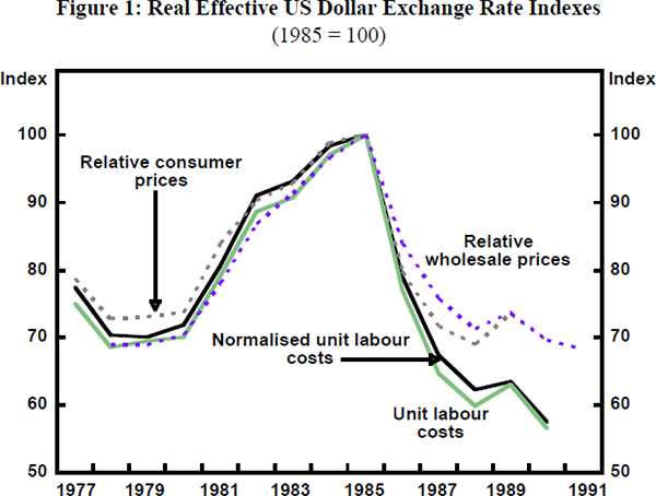
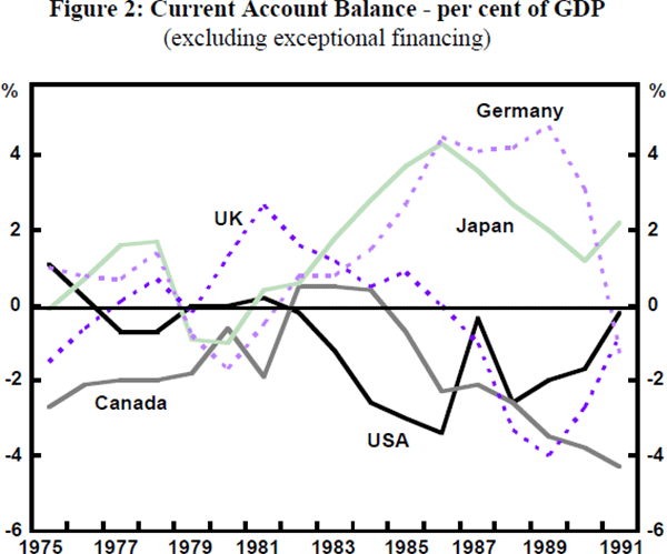
Figures 1 and 2 show, respectively, that the depreciation of the real effective $US rate since 1985 – however measured – has been substantial, and that there has been, subsequently, a clear turnaround in the US balance of payments deficit with corresponding changes in the external accounts of Germany and Japan. Earlier impatience with the slowness of the turnaround has been revealed for what it was – impatience. In substantial degree, the contributions to Bergsten's (1991) review of the period suggest that the basic theory of international adjustment has survived well.[3] However, it is less than clear how much of what is satisfactory about the outcome should be attributed to the Plaza process itself, rather than to other factors. There is the point that the $US was already falling, ahead of the Plaza agreement itself and, in fact, had gone the whole distance initially desired within a month of that agreement. There were substantial shocks during the period – the fall in oil prices in 1986, the stock market crash and German reunification. Also, there are some doubts about the way in which the process was made effective.
2.3 Instruments and Implications for Monetary Policy
The rhetoric of the Plaza process laid great emphasis on the combined use of three instruments of policy – intervention in the foreign exchange markets, monetary policy and fiscal policy. One seemingly very important finding to emerge from recent studies (see Catte et al. (1992a, 1992b)) of the Plaza episode is the significance attached to foreign exchange market intervention. Prior to this, the conventional wisdom of both academics and policy makers was that intervention per se (sterilised intervention) could not be important, except for any signals it might convey about monetary policy (that is, about unsterilised intervention), a caveat that came to be treated as rather unimportant. This followed from the demonstration that if assets of different currency denominations are perfect substitutes, then sterilised intervention could not change the exchange rate, and also from a general presumption that ‘perfect substitutability’ would not be a bad characterisation of G5 currency-denominated assets (Obstfeld 1983). Mussa (1981) supplied the qualification about the possible signalling role of intervention. At the same time, the Jurgensen Report (1983), which was inspired by the Versailles Summit, conveyed a similar message to policy makers. By contrast, the more recent studies of intervention suggest that, since 1984, all but one of the major turning points in the trajectory of the $US exchange rate coincide with episodes of intervention and that over half of the episodes of concerted intervention (involving at least two of the G3) since 1984 were definitely successful, with the remainder registering temporary success. As Williamson (1993) notes, this ‘new view’ of the effectiveness of intervention sits better with theories that give much room in short-run exchange rate determination to fads and bubbles, than with theories which emphasise the fundamentals; for, in the former case, it is possible to argue that the markets have very little to go on and thus may be ‘given a steer’ by official intervention. It would also be wise to concede, though, that studies of this period are as yet few and do not amount to a consensus. (For example, the study by Kaminsky and Lewis (1993) arrives at fundamentally pessimistic conclusions about the usefulness of intervention. Although intervention has information content, these authors find that the signal is actually perverse.)
Nevertheless, sterilised intervention was not sufficiently effective to avoid pressures arising on monetary policy.[4] Among the criticisms of this policy episode are, in fact, the following points: that fiscal policy was relatively unresponsive to the demands of coordination, putting ‘too much’ of the burden on monetary policy; that the distribution of this burden was essentially decided in the interests of the United States; and that overall monetary policy was probably too lax, prolonging the life of the global stock market ‘bull run’ and making inevitable at some point a stock market crash of the kind that did, in fact, eventuate. The crux of the argument is the following simple point. The proximate determination of the exchange rate is a function of relative interest rates. (Following the Plaza Accord, to ensure that the $US fell, but not too fast, US interest rates needed only to lie below rates in Germany and Japan by a judicious margin.) But this does not determine the absolute level of interest rates. (This was left to the United States.) For domestic reasons, the United States wished to see low interest rates at home; it left other countries to determine the exchange rate. Funabashi (1989) is very revealing in this regard. Commenting on US policy through 1986, he says ‘The Fed used monetary policy to stimulate the US economy or at least to keep it buoyant but it did not burden monetary policy with exchange rate management. Instead it used coordination of monetary policies – more accurately, the monetary policies of others – to keep the dollar from dropping precipitously’ (Funabashi 1989, p. 57). It is arguable that the absolute level of interest rates to which this led, at least in Japan, was undesirably low, prolonging the overvaluation of the stock market. Also, it seems that it was conflict with Germany over the level of interest rates (with Germany's policy concerns pointing to higher levels than implied by US policy concerns) that led, proximately, to the crash.
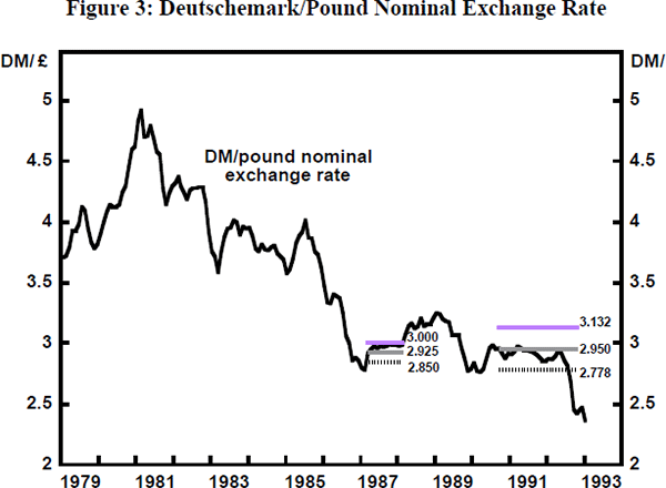
In the United Kingdom, the episode was used by Chancellor Lawson as cover for an experiment in ‘shadowing’ the DM, presumably designed as a way of showing that full-blown membership of the Exchange Rate Mechanism (ERM) could be easily managed. ‘Unofficially’, it was made clear that the UK authorities were targeting the deutschemark (DM) to a ceiling of 3DM to the pound. The policy is unmistakable in the data (see Figure 3).[5] At this time there were gathering signs of inflationary pressure in the United Kingdom, which would have suggested increases in interest rates; yet sentiment was very favourable towards the pound and maintaining the exchange rate below the ceiling meant foregoing such increases. The incident can be recognised as a forerunner of the ‘excess credibility’ problem (see below) experienced by some other ERM countries in the late 1980s and early 1990s. After about a year, the policy was abandoned in the face of mounting inflationary pressure and the exchange rate rose through its erstwhile ceiling.[6] The Plaza episode may have been successful in its major objectives and sterilised intervention appears to have been an important and effective part of the policy toolkit. However, there were monetary implications, especially for countries other than the United States, which do not seem to have been so obviously desirable. Admittedly, in the case of the United Kingdom, the monetary consequences were essentially self-made, a product of a substantial ‘hardening’ of the Plaza-Louvre process rather than of the process itself.
Whilst participants in the coordination process inaugurated by the Plaza Agreement refrained from issuing publicly stated exchange rate targets and bands, the process involved was recognisably of this genre. This is one reason why it is interesting to examine the choice of target exchange rate more formally; another reason why this is of interest arises quite naturally from the partial collapse of the ERM in September 1992. Was this the consequence of destabilising and destructive speculation? Or was the crisis revelatory of fundamental disequilibrium? How can we recognise when an exchange rate is away from its equilibrium?
3. Williamson's FEERs
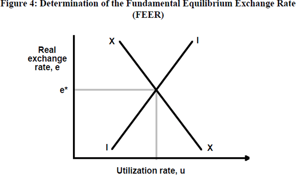
The academic ‘blueprint’ closest to the spirit of the G5 intervention was that produced by Williamson (Williamson 1985a; Edison, Miller and Williamson 1987; Miller and Williamson 1987). His proposals centre around the suggestion that a ‘fundamental equilibrium exchange rate’ (FEER) should be identified and targeted within a ‘soft-edged’ band. The FEER is that rate of exchange which is consistent over the medium term with internal and external balance. Clearly this is a real rate of exchange. The FEER is, in principle, a trajectory, or exchange rate path. Expressed in nominal terms, any given FEER trajectory would need to be adjusted additionally for relative inflation.
Clearly, identifying such a rate is far from being a straightforward task in principle: Williamson emphasises that a broad error band (plus or minus 10 per cent) must be associated with his estimates. In the simplest settings, internal balance is independent of the real rate of exchange, but in rather open economies this is not likely to be the case (Wren-Lewis et al. 1990). In the diagram (Figure 4), for example, a Layard and Nickell (1985) ‘battle of the mark-ups’ view of inflation makes the internal balance schedule (II) slope up from left to right in exchange rate-utilisation space. The external balance schedule (XX) slopes down from left to right for obvious absorption-elasticity reasons. The FEER is located at the point of intersection of the two schedules.
The FEER suffers from hysteresis. If the actual exchange rate is not at its FEER value then the balance of payments (given internal balance) will differ from that implied in the calculation of the FEER. However, this in turn, implies a different external debt and debt-service trajectory from that implied in the original calculation, so the FEER should be recalculated.[7] To be concrete, suppose that the exchange rate is appreciated relative to the FEER – then the FEER should be devalued relative to its original value in order to protect the external account from the increased volume of debt-service payments otherwise implied. Artis and Taylor (1993a) have expressed this problem in analytical terms, simulated it on historical data and derived some ‘rule of thumb’ adjustments that can be made to take care of it. The problem, whilst real, seems to be a manageable one.
Another problem with the FEER is the assignment issue. Since the FEER itself is a real rate, a potential criticism would be that it accommodates inflation. In the full blueprint, Miller and Williamson circumvent this criticism by adding an additional target, for nominal domestic demand. Then (real) interest rates and intervention target the FEER, whilst fiscal policy is used to target the nominal demand objective. In a symmetric system, this still leaves it open for the collective of participant countries to target a global price level by coordinating their national nominal demand targets. Whilst logically complete, the assignment may be criticised on the grounds that in practice the required flexibility of fiscal policy does not exist: thus practical implementation of such a scheme (as in the G5 experience) would simply lead to over-emphasis on monetary policy.
Finally, though termed the ‘fundamental’ equilibrium exchange rate – echoing the Bretton Woods provision for exchange rate adjustment in circumstances of ‘fundamental disequilibrium’ – it is clear that there is a normative edge to the concept of the FEER which some critics, such as Frankel (1987) find oppressive. The point is that the estimates of internal balance from which the FEER is derived are constructed as medium-run sustainable positions. This deliberately ‘rules out’ the use of discretion by governments to follow temporarily unsustainable policies. In his reconstruction of the logic of the Bretton Woods system, Williamson (1985b) is absolutely clear that it was a virtue of that system that commitment to exchange rate stability ruled out irresponsible policy, and it is equally clear that this virtue is intended to be embodied in the FEER blueprint.[8] Significantly, in simulations of the world economy with FEERs in place and Williamson-Miller policy assignments, Currie and Wren-Lewis (1988) found that the US fiscal ‘experiment’ of the 1980s was essentially wiped out. However, recent events in the EMS found analysts looking for a concept of the equilibrium rate of exchange against which to measure desirable adjustments and the FEER is much the best articulated measure.
4. Nominal Exchange Rate Targeting
Basic analytics indicate that there are a limited number of nominal variables that might in principle serve as ‘nominal anchors’, in the sense that success in stabilising them would imply success in stabilising the price level. They include the nominal wage, the money supply, the nominal exchange rate and prices directly (the ‘Antipodean anchor’). Well-known policy episodes correspond to each of these. In simple models, the exchange rate is the dual of the money supply: the monetary implications of exchange rate targeting supply are very clear in this case. The exchange rate target implies the endogenisation of monetary policy. Even in models where one-to-one correspondence fails, the general spirit of the implication still holds: while the exchange rate target prevails it will not be possible to execute an independent monetary policy (except in the case where sterilisation is feasible – an important issue in the case of the EMS, as discussed below).
Nominal exchange rate targeting may be followed in a variety of forms, from ‘strong’ to ‘weak’ and in a variety of political contexts. Outright commitment to a nominal peg is nearly always hedged by a band around the central rate; this ‘strong form’ exchange rate targeting may take place on the basis of go-it-alone commitment to a peg against a basket or a single currency – an alternative is that commitment takes place inside an exchange rate union of participating countries (the EMS example). Motivating economic arguments here have commonly invoked the ‘credibility model’ of economic policy, to the point where the exchange rate peg is conceived of as a way of ‘importing the credibility’ of the central bank of the currency against which the peg is maintained. How this can be better than alternative ways of earning credibility is one of the issues reviewed below.
By ‘weak form’ exchange rate targeting we mean, for want of a better phrase, situations in which the exchange rate is viewed as an important conditioning variable on monetary policy responses, although there may be no public (or perhaps even private) target for it. Weak form targeting seems to be a common practice amongst countries which have tried and found wanting either a monetary targeting style of policy or a strong form exchange rate target.
A standard result in the literature on the relative merits of monetary and exchange rate targeting is that each regime is uniquely vulnerable to certain types of shock. As shocks alternate over time, the optimal policy may be a switching regime; the change from a monetary target to an exchange rate target in Switzerland in 1978 is a well-known example. The weak form exchange rate targeting regime is a generalisation, where the response to monetary target overruns may be conditionalised on the exchange rate. This is, in effect, what occurred in the United Kingdom in the early to mid-1980s as Prime Minister Margaret Thatcher's monetarist experiment was relaxed in the face of the unprecedented appreciation of the pound sterling. More recently (as discussed below), it has become more fashionable to emphasise the direct targeting of inflation using the central bank's policy instrument (an interest rate): but such a policy may be prosecuted (as currently in the United Kingdom) in the context of concern for the evolution of both the money supply and the exchange rate.
It might be expected that studies of the transmission mechanism of monetary policy would emphasise the role of the exchange rate. After all, one natural way of justifying exchange rate targeting would flow from a picture of that transmission mechanism as m → e → y, p with the link between m and e being uncertain and ‘fuzzy’. Then exchange rate targeting simply cuts out the ‘unreliable’ part of the transmission mechanism. We attempted to investigate this issue, using measures of linear feedback developed by Geweke (1982, 1984). The results, which are reported in full in Appendix A, appear distinctly disappointing for those of the view that the exchange rate is a significant part of the transmission mechanism of monetary policy.
In what follows below, we take a look at weak form exchange rate targeting of the type described above, as exemplified discontinuously over recent years in the United Kingdom. Then we examine the situation of participants in the ERM of the European Monetary System.
5. ‘Weak Form’ Nominal Exchange Rate Targeting
The practice of considering the exchange rate to be an important conditioning variable for counter-inflationary policy stems from the basic mark-up model of pricing and the view that nominal wages tend to adjust for price changes. Then it is easy to show that a nominal devaluation of the exchange rate will tend to feed into increases in domestic wages and prices. Of course, this is a price level adjustment rather than inflation per se (except in the case that the devaluation itself is continuous), but from the short-run policy view involved here, the distinction may be uninteresting. With a view to completeness and clarity, though at some risk of being obvious, we spell out the basic mark-up model and illustrative simulations in Appendix B.
Given the view that nominal interest rate adjustments can have significant effects
on demand independent of their effects on the exchange rate, and thus influence
prices (both through excess demand impacts in the labour market and by changing
the mark-up), a trade-off emerges between interest rate adjustment and exchange
rate changes. If the exchange rate appreciates, interest rates can fall, consistent
with an unchanged inflationary pressure. If the exchange rate depreciates,
then interest rates must be raised to preserve the same counter-inflationary
stance of policy. This account of matters gives privilege to the interest rate
as the monetary policy instrument, which is the way central bankers tend to
think about the problem. These considerations can be usefully presented in
a diagram (Figure 5) in interest rate-exchange rate
space.[9]
The exchange rate is measured as the number of units of domestic currency per unit
of foreign currency, so an increase indicates a devaluation. Then the schedule
 = 0
indicates an iso-inflation objective line. The more devalued the currency, the higher
the interest rate needs to be to prevent the inflation rate rising. An appreciated
currency allows the central bank to ease interest rates. Points to the right
and below the schedule represent points of relative inflation, points to the
left and above indicate relative deflation.
= 0
indicates an iso-inflation objective line. The more devalued the currency, the higher
the interest rate needs to be to prevent the inflation rate rising. An appreciated
currency allows the central bank to ease interest rates. Points to the right
and below the schedule represent points of relative inflation, points to the
left and above indicate relative deflation.
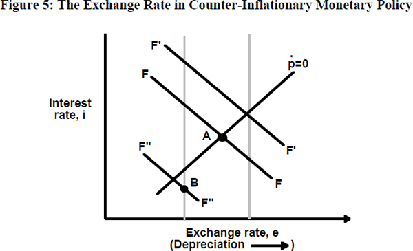
The schedule FF is a foreign exchange market schedule, assumed to slope down from
left to right, so that a high interest rate is associated with an appreciated
exchange rate and a low one with a depreciated rate. A shift in foreign exchange
market sentiment – say, a reaction to unfavourable news – would
shift FF to a position like F′F′. If interest
rates are not raised this would lead to inflation. Staying on = 0 requires
interest rates to be increased. The diagram can be used to describe the problem
encountered by Chancellor Lawson when he decided to ‘harden’ his
policy and to target the DM exchange rate (as described above). The dashed
vertical lines represent the bands around the commitment on the exchange rate.
Suppose now that the foreign exchange market views the new developments very
favourably, or for some other reason moves into the pound sterling. Then FF
could shift to a position like F″F″, and in order to prevent
the exchange rate from appreciating through the ceiling, the interest rates
will have to be set, as at point B, on the ‘inflationary’
side of = 0. Although
the exchange rate commitment is intended as a ‘hard’ counter-inflationary
policy, the result here is ‘excess’ inflation.
The policy of conditioning monetary policy responses on the exchange rate, as opposed to outright exchange rate targeting, has a number of virtues. It avoids the problem of ‘excess credibility’ just illustrated and it provides no hostages to fortune. It is flexible in allowing the authorities to adjust policy in the light of circumstances, but it is just this which critics will attack. The policy can have no credibility other than what is earned through the results as reflected in the control (or otherwise) of inflation. There is no other nominal anchor. By comparison, the credibility model of economic policy has been a dominant point of appeal in reconstructions of the benefits of participation in the ERM.
6. Participating in the ERM
Until the near-collapse of the ERM of the European Monetary System last year, it seemed possible to describe it as an outstandingly successful arrangement. Certainly, new countries joined it with enthusiasm; Spain in 1989, the United Kingdom in October 1990 and Portugal in 1991. Some countries not eligible for formal membership (Austria and the Scandinavian fringe) also signed up informally by targeting the DM or the ECU. The chief motivation for joining was a belief in the counter-inflationary benefits that could be gained. Economic theory provided some basic building blocks. One can identify three such blocks. Starting with the most basic of all, there is the mark-up pricing model, together with a real wage resistance view of wage inflation.[10] Then, there is the demonstration that, for equal degrees of credibility, an exchange rate target is just as good and probably better than a monetary target for delivering low inflation (Artis and Currie 1981). Finally, there is the credibility model of counter-inflationary policy, such as Barrro and Gordon (1981), which could be interpreted to promise that some differential credibility would attach to an exchange rate targeting strategy, particularly one conducted in the context of an international arrangement. (The differential credibility stems from the visibility of the exchange rate and from the assumption that the ‘punishment’ for reneging is strengthened in such a context.) The predictions that could be derived from these component assumptions seemed to be borne out in the late 1980s and early 1990s. Exchange rate volatility between ERM member currencies had fallen; no realignments had taken place since 1987 (aside from the ‘technical’ realignment implied by Italy's decision to move from her ‘broad’ band (plus or minus 6 per cent) to the ERM narrow band (plus or minus 2.25 per cent) whilst keeping the same ‘floor’ rate as before). Inflation had fallen and converged, while the dispersion across ERM countries narrowed. All this appeared to result from the fact that whilst the ERM statutes described a symmetric system, the practice had been markedly asymmetric, centring on a low-inflation Germany as the leader or hegemon of the EMS.
We now turn briefly to describe the formal arrangements of the EMS and its practical evolution.
7. Formal Provisions of the EMS
The heart of the EMS is the exchange rate mechanism. Participation in the mechanism obliges a country to maintain its bilateral parity against other participants within pre-agreed bands around a central rate. Formally this obligation falls on both sides, that is, equally on the strong and on the weak currency country. Credit is provided to support intervention in the foreign exchange market very short term facility (VSTF); in 1987, when the original (1979) provisions were amended following the so-called Basle-Nyborg agreements, the credit lines were extended to foreign exchange market intervention within the bands (so-called ‘intra-marginal’ intervention) and the repayment period was lengthened. The impression of symmetry was further strengthened by the ‘invention’ of a unit of account (the ECU), in which exchange rates could be expressed and credits denominated. The existence of the ECU made possible the design of the ‘divergence indicator’; when a country's ECU rate departs from its central parity by an amount that represents a shift against other currencies of 75 per cent of the 2.25 per cent permitted deviation,[11] then a presumption falls on that country to take diversified corrective action.
Such action could include measures of fiscal and monetary policy, intervention and a realignment of the central parity of the currency.
8. Practical Evolution
In practice, the EMS evolved as an asymmetric system, with Germany as the leader and the DM as the anchor currency. A proximate explanation for this is that the leading policy concern of the 1980s was that of inflation. The conversion of the EMS to an asymmetric system emphasising counter-inflationary policies was gradual. In the early years, there were many realignments and in that period the EMS behaved somewhat like a crawling peg. This gave way after around 1983 (the year of the ‘Mitterand U-turn’) to the asymmetric model.
A stylised description of how the asymmetry and the counter-inflationary bias of the EMS worked out in practice would emphasise the following features. Firstly, Germany typically abstains from all intra-marginal intervention and aims to sterilise the consequences of obligatory, marginal, intervention (Mastropasqua, Micossi and Rinaldi 1988). Secondly, realignments became a matter for multilateral decision (Padoa-Schioppa 1983), with a bias towards ensuring that exchange rate devaluations ‘underindex’ on cumulative relative price differentials (Padoa-Schioppa 1985). Thirdly, the divergence indicator fell into desuetude (it would have been contrary to the counter-inflationary objective to have insisted that the low inflation leader should expand). Thus, on this stylised view, Germany pursued her own monetary policy where other countries, by contrast, were in the position of accepting the German lead. Any difficulties they might have had in doing so were reduced (for those countries which had them) by the use of capital exchange controls (France and Italy).[12] The decision to phase out those controls, followed by their gradual and eventual total removal, marked the beginning of a new phase in the history of the EMS, that of the so-called ‘New EMS’.
The outstanding characteristic of the ‘New EMS’ is that, up until the crisis of 1992, realignments ceased to take place.[13] This outcome is in contrast to the suggestion emanating from the Basle-Nyborg discussions, to the effect that in the new conditions of greater capital mobility, smaller and more frequent realignments would be called for. The suggestion was that destabilising speculation could be avoided if realignments were adopted in timely fashion and came in amounts less than the band width of the currency concerned, so that the market rate would not be disturbed. In this way, the ‘one-way bet’ would be avoided. Some analyses see this as the fatal mistake which led to the debacle of 1992.
It is this last period and the events leading up to that debacle that are of greatest interest and they will occupy the remainder of the paper.
9. The ‘New EMS’
The policy apprehension at the start of the period designated the ‘New EMS’ was not at all like the immediate outcome. The tone of the debate at that time was that the removal of capital controls would expose the follower countries to sharper policy pressures: policy dilemmas – whether to follow Germany or to attend to domestic objectives – would be more acute. It did not seem accidental that the revival of pressure for a move to European Monetary Union, within which framework countries could share decision making with Germany, came about at this time. Meanwhile, if speculators sensed that the policy makers were facing sharper policy dilemmas, they would test the System's ability to hold exchange rates constant. A symposium in the May 1988 issue of The European Economy is symptomatic: one author took the view that the new conditions warranted wider bands, others that exchange controls should be reinstated. It was easy to agree that realignments that were small enough to be accommodated within the bands and thus without disturbing the market rate were to be encouraged; and that more cooperation between the monetary authorities of the EMS countries would be necessary. Driffill (1988) argued that with suitable combinations of domestic policy discipline, interest rate policy coordination and ‘small’ realignments the EMS should be capable of surviving without exchange controls.
The EMS did, in fact, survive without realignments until 1992. Exchange rates could still have been quite volatile within the bands; or exchange rate stability could have been bought at the expense of increased interest rate volatility. In fact, it seems that volatility of both exchange rates and interest rates continued to decline (Artis and Taylor 1993b). On the other hand, a slowing down in the reduction of inflation and its convergence seemed to become obvious.
A policy perversity exhibited itself in particular cases (Italy for a while, Spain more noticeably) which gave rise to Alan Walters' famous description of the System as ‘half-baked’. Whilst a sizeable dispersion of inflation still persisted, the credibility of the exchange rates was tending to bring about a convergence of nominal interest rates. This suggested that real interest rates might be lower in the higher inflation countries than in the low inflation countries – a perverse ranking. Giavazzi and Spaventa (1990) called this ‘excess credibility’, presumably because the exchange rate credibility is not consistent with divergent inflation: at some point in the future, the exchange rates would need to be changed to correct the cumulative misalignments (Miller and Sutherland 1991). A transitory problem may nevertheless be one of serious magnitude for policy makers over a significant period of time. This is how it appeared in this case.
A very simple model of the ‘Walters Critique’ may be set out in the following way:
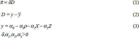
Equation (1) specifies that inflation (π) will accelerate in the presence of excess demand. Otherwise
it will proceed at its core (inertial) rate. Excess demand is specified in
equation (2) whilst equation (3) shows aggregate demand as inversely related
to the real interest rate (ρ), the real exchange rate (X) and
a vector of other policies, suitably scaled, Z. The country is small
relative to Germany. The real exchange rate is measured relative to the DM
and equilibrium is where  (German inflation)
and the real exchange rate is at its equilibrium value (
(German inflation)
and the real exchange rate is at its equilibrium value ( ). The nominal exchange
rate is assumed to be fixed.
). The nominal exchange
rate is assumed to be fixed.
In Figure 6 the horizontal line drawn at π = πg
is also the schedule corresponding to  = 0 where
the real exchange rate is not changing, as prices in Germany and the ‘home
country’ are rising at the same rate. The schedule
= 0 where
the real exchange rate is not changing, as prices in Germany and the ‘home
country’ are rising at the same rate. The schedule  = 0 is a schedule
of zero excess demand. If nominal interest rates are forced, by ‘excess
credibility’ to German levels, then a rise in inflation will reduce real
interest rates and raise excess demand. To offset this, the real exchange rate
must rise. So the = 0 schedule
would slope forward, as shown. This system is not
stable (see Appendix C);
but if nominal interest rates rise by more than the inflation rate, insuring that
real rates rise with inflation, the system can be stabilised. The system, of
course, can always be ‘made stable’ even in the presence of excess
credibility, if ‘other policies’ (Z) are used so
as to exert deflationary pressure as inflation rises.
= 0 is a schedule
of zero excess demand. If nominal interest rates are forced, by ‘excess
credibility’ to German levels, then a rise in inflation will reduce real
interest rates and raise excess demand. To offset this, the real exchange rate
must rise. So the = 0 schedule
would slope forward, as shown. This system is not
stable (see Appendix C);
but if nominal interest rates rise by more than the inflation rate, insuring that
real rates rise with inflation, the system can be stabilised. The system, of
course, can always be ‘made stable’ even in the presence of excess
credibility, if ‘other policies’ (Z) are used so
as to exert deflationary pressure as inflation rises.
The systemic performance of the ‘Walters Version’ of this model, however, is not borne out in the empirical results quoted in Table 1. The hypothesis is that the ranking of countries by inflation should be negatively correlated with the ranking by real interest rates in the ‘New EMS’ period. What the table shows is that this correlation is significantly negative for the ‘Old EMS’, but positively correlated (not always significantly) for the ‘New EMS’. Different sample separations are used, to accommodate the arbitrariness of dating the switch in regime. (The exclusion of Denmark simply dramatises the results.) The negative correlation for the ‘Old EMS’ is, in fact, not surprising when the presence of capital exchange controls is borne in mind. Such controls broke the arbitrage nexus between onshore and offshore markets and enabled interest rates to be held at ‘artificially’ low levels. Whilst the Walters problem does not appear to have been of systemic significance according to these results, it nevertheless seems clear that for certain countries (notably Italy and Spain) excess credibility was a real problem It was a contributor to the overvaluation revealed by the events of September 1992.
| 79:4– 82:12 |
83:1– 91:12 |
79:4– 84:12 |
85:1– 91:12 |
79:4– 86:12 |
87:1– 91:12 |
|
|---|---|---|---|---|---|---|
| ERM 6 countries including Denmark |
−0.60(b) | 0.73(b) | −0.47 | 0.73(b) | −0.07 | 0.47 |
| ERM 5 countries excluding Denmark |
−1.00(a) | 0.60 | −0.80(b) | 0.60 | 0.00 | 0.40 |
| Notes: (a) Indicates rejection of the null hypothesis at 1%. (b) At 5% and at 10% (one-sided test), where H0 is zero correlation and H1 is negative or positive correlation depending on the sign of τ. (c) ERM 6 is France, Germany, Netherlands, Belgium, Italy and Denmark. Denmark was omitted in ERM 5 owing to doubts about the comparability of the data. |
||||||
10. The September 1992 Crisis
The September 1992 crisis, which saw Italy and the United Kingdom forced to float freely and also brought about devaluation of other currencies led to a period of currency instability inside the EMS (Table 2). Nearly every currency was ‘attacked’ and only four survived – the French franc, the Dutch guilder, the Danish Kroner and the Belgian franc. Why did these currencies survive and what does the crisis hold in store for the future of the EMS?
| 1992 | |
|---|---|
| September 12th | Lira devalued by 7 per cent |
| September 16th | Pound sterling floated |
| September 17th | Lira floated Peseta devalued by 5 per cent |
| November 22nd | Peseta devalued by 6 per cent Escudo devalued by 6 per cent |
| 1993 | |
| January 30th | Irish pound devalued by 10 per cent |
| May 13th | Peseta devalued by 8 per cent Escudo devalued by 6.5 per cent |
The proximate events to set off exchange rate pressures were, as is well-known, the negative Danish referendum rate on EMU and the unemphatic French referendum result (the so-called ‘petit oui’). The ‘fundamentals’ had not moved suddenly beforehand to precipitate the crisis.
There seem to be two main explanations. In one, the argument is that the fundamentals had gone wrong for several major currencies and that some smaller currencies were likely to be implicated as a ‘domino effect’ in the consequent correction (for example, the Irish pound would likely need to be devalued in the face of a devaluation of the pound sterling, and similarly the escudo, in the case of the peseta). In this argument, the timing of the collapse has to be assigned ‘minor’ significance. The misalignment of fundamentals is a cumulative process and had already reached a critical point. Any sign that governments might not be so keen to defend central parities would have sparked a crisis. In the alternative explanation, the precipitating events are crucial, in that they reveal a distinct probability of an alternative equilibrium. The fundamentals are endogenous.
There are also two other factors to be considered explicitly: the role of the German unification shock on the one hand; and the role of the Bundesbank on the other.
Let us look at these factors immediately. The unification shock, particularly given the way in which Germany chose to handle it (involving a large fiscal expansion and tight money) was a textbook case of an asymmetric shock requiring a real appreciation of the DM. This could be accomplished in one of two ways: without a nominal appreciation of the DM by relative deflation outside Germany; or, with a nominal appreciation to assist the process. The difficulty of the relative deflation requirement is that Germany's inflation aversion sets a low ceiling to the absolute rate of inflation in Germany, thus forcing a particularly low inflation requirement on other countries. The Bundesbank reportedly offered the prospect of a general realignment to her EMS partners. Why was the offer not accepted? A proximate answer appears to lie in a combination of over-adherence to the credibility model and a classic cooperation problem. The credibility model was seen as requiring that no nominal devaluations should be undertaken. However, a general realignment could have been presented in such a way as to minimise the loss of credibility. But since one country, France, vigorously refused to contemplate such a realignment, other countries were, in effect, forced to consider only the possibility of individual exchange rate depreciation. This maximised conflict with the credibility requirement and so the option of pre-emptive realignment was abandoned.
A second important issue here is the role of the Bundesbank. It is readily observable that where the Bundesbank chose to pledge its commitment to defend the French franc/DM rate, that rate survived. Simply put, since no-one has more DM than the Bundesbank such a commitment is bound to defeat even determined and well-financed speculators. A literal reading of the EMS statutes suggests, however, that a commitment to infinite intervention at the margins is an important part of the system, something which all participants can rely on. The speculative crisis has drawn attention to the fact that in the early days of the EMS the Bundesbank obtained an assurance from the German Government that it could be released from such an obligation if the commitment should appear to undermine the Bundesbank's ability to maintain stability of the currency domestically. No-one knows whether this escape clause was invoked during the crisis – or was about to be invoked, which is really all that is necessary.[14] However, reflection clearly suggests that no central bank could afford to accept an obligation of unlimited intervention against weak currencies. This would be to run the risk of not only underwriting the inflationary impulses of a weak currency country, but of importing those impulses via a continuous increase in the money base and thereby increasing prices. Under the operating conditions of an earlier decade these issues were not so obvious. Capital controls and realignments kept them at bay. At higher absolute levels of inflation the need for individual countries to accept stabilisation packages was usually more obvious. Most intervention was intra-marginal and the Bundesbank did not participate in this type of intervention.
The combination of overvaluation, discrepant policy cycle and ‘domino effect’ goes a long way – arguably sufficiently far – towards explaining the crisis.
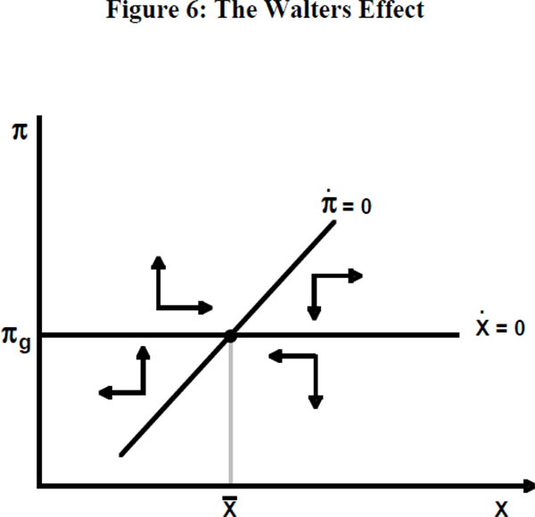
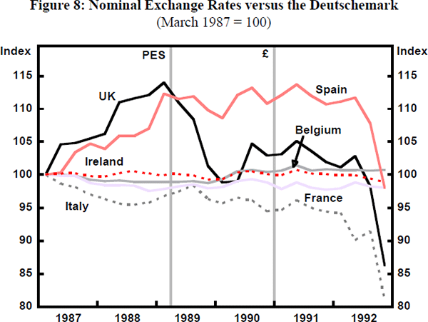
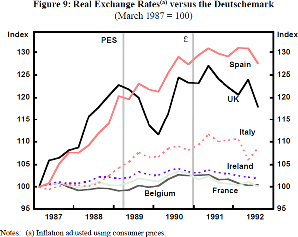
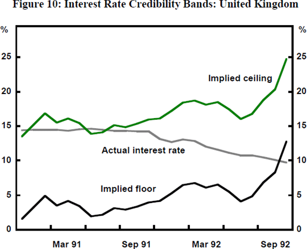
Figures 7, 8 and 9 illustrate the argument with respect to competitiveness. It seems clear that cumulative inflation differentials, combined with an absence of nominal exchange rate adjustment, produced overvaluation in the lira and peseta. At least, if these currencies were locked in at the ‘right’ exchange rate earlier, that exchange rate had become overvalued by 1992. However, this does not go far enough. The position of Ireland does not seem to be explained by overvaluation. Here, two other factors must be brought in. The first is the ‘domino’ effect. Trade with the United Kingdom is sufficiently important for Ireland that a sizeable pound sterling devaluation must create a presumption that the Irish pound is overvalued. (The domino argument goes for the Portuguese escudo also.) The second factor, important also for the United Kingdom, is the ‘policy cycle factor’. A country that maintains its competitiveness by deflationary policies may increasingly be suspected of nearing the point at which its commitment to peg its currency will be abandoned. The UK Government had understood that pegging to the DM could introduce policy conflict but its appreciation of the extent of such conflict was too sanguine. In its 1991 restatement of the Medium Term Financial Strategy it stated that: ‘There may be occasions when tensions rise between domestic conditions and ERM obligations, with domestic conditions pointing to interest rate levels either higher or lower than those indicated by ERM obligations’. The problem is, of course, that when a devaluation is in the offing, the choice is not between an interest rate at German levels and an interest rate at lower levels, but between a rate which is quite possibly a multiple of the German rate and the more desirable lower rate.[15] In fact, United Kingdom interest rates were maintained well within the ‘credibility bands’ (see Figure 10)[16] until the edge of the crisis was reached, though it is noticeable that the rate is slipping towards the floor value from before the beginning of 1992. The continued rise in unemployment in the United Kingdom increasingly made it appear that the commitment could be shaken.[17] Something of the same kind could also be said for Ireland. For the United Kingdom, also, it is important to note that the best available estimate of the fundamental equilibrium rate suggested that the DM parity was some 20 per cent overvalued upon entry (Wren-Lewis et al. 1990).
The combination of overvaluation, domino effect and asynchronous policy cycles can account, it would seem, for the major devaluations and crisis casualties. The problem, from this point of view, is more in explaining why the system had been so stable while these misalignments were building up.
The suggestion put forward by Eichengreen and Wyplosz (1993) attempts to tackle this issue. They argue that the system was essentially one of multiple equilibrium. Their argument is that the convergence criteria in the Maastricht Treaty and the anticipation of an early move to EMU maintained in speculators' minds the probability that governments would pursue highly disciplined policies. Once the Danish and French referendum results undermined this assurance, the probability that countries would pursue less disciplined policies became real. A successful raid on a currency would force that currency off the EMU track and make it more likely that discipline would be relaxed. Forward-looking exchange rate fundamentals are, in effect, endogenous. A successful raid shifts the fundamentals in a manner which ‘justifies’ the raid.
It seems that the two approaches are, in fact, complementary. The fact is that whilst most currencies were attacked, not all succumbed. For those that did, an explanation based on a combination of over-valuation, policy cycle and domino effects makes good sense. But clearly there is a ‘timing problem’. The multiple equilibrium approach helps rationalise the timing but does not explain why not all currencies were successfully attacked.
11. The Sequel: A Two-Tier Solution?
In the minds of many observers the crisis of 1992 has underlined the relevance of a ‘two-tier’ sequel. An inner group (Benelux, France, Germany and Denmark) may narrow their margins and may proceed directly to EMU under the Maastricht ‘two-tier’ clause. An outer fringe may maintain wider margins and a slower timetable for participation in EMU.
There are two points of interest worth commenting upon in such a potential solution. Firstly, there is the issue of how far the Bundesbank is capable, under present conditions, of maintaining its ‘own’ monetary policy, let alone providing adequate leadership. Broad consideration of the extent of currency substitution within the inner tier and the difficulties of sterilisation in open capital markets provide reminders that substantial doubts must exist in both respects.[18] The second point of interest is that the setback experienced by the outer fringe of countries – including the destruction of their stock of credibility – does not yet seem to have significantly lessened their commitment to exchange rate targeting. This must underline the findings of Honkapohja and Pikkarainen (1992) to the effect that the attachment to ‘fixity’ of the EMS countries owes more to political than economic factors. The long stop is that the achievements of the EC in dismantling protectionism between member countries require some kind of real exchange rate stability. With appropriate arrangements for flexible adjustment this has so far been seen as creating a bias in favour of nominal fixity. Nevertheless, in the immediate future, exchange rate promptings are going to be less insistent in influencing the conduct of monetary policy than they have been in the recent past for this group of countries. There is certainly scope for improvement in the conduct of monetary policy; whether it will be realised has to remain another question.
Appendix A: The Transmission Mechanism of Monetary Policy in a Causal Framework
A.1 Introduction
The nature of the transmission mechanism of monetary policy and its stability remain important issues for investigation. In a number of countries, the 1980s witnessed a process of liberalisation which might have been expected to alter the characteristics of the transmission mechanism. Artis (1992) represents an attempt to comment on this issue by examining the stability of measures of unconditional linear feedback connecting monetary variables to output and prices (Geweke 1982, 1984). Covering the United States, the United Kingdom, Italy, France and Germany, that study found less evidence of disturbance to some of these relationships than might have been expected.
Accordingly, in this Appendix, an attempt is made to carry the analysis further. By focusing on measures of conditional linear feedback (also introduced by Geweke (1984), it should be possible to identify some characteristics of the transmission mechanism – for example, whether money affects prices via the exchange rate or in some other way.
Two important restrictions on the nature of this exercise can be stated as follows. Firstly, the measures that are used presume a predominantly causal structure to the monetary process and our interpretation is conditioned accordingly. Secondly, it will become apparent that in effect, what we are doing is translating from statements about the information content of variable x for predicting variable y in the presence of information on variable z to statements about the actual causal structure of monetary processes, in which x may be described as influencing y through z (or not, as the case may be). The term ‘transmission mechanism’ is used here, then, in a precise technical sense, rather as, in a similar way, the term ‘causality’ has been employed before in related studies.
The methods used to isolate the transmission mechanism rely on an assumption that the underlying data series are stationary and it is usual to find that investigators work with log-differenced time series data for this reason. Thus the relationships estimated resemble the dynamic second-stage equation from the Engle-Granger two-stage cointegration procedure, with the omission of the error-correction term (lagged residual from the first stage cointegration equation). If the variables in question are in fact cointegrated at the first stage, this omission would represent a misspecification of the true relationship. In such situations, as Granger (1988, p. 204) has noted: ‘It does seem that many of the causality tests that have been conducted should be re-considered’.
We therefore take care both to check for the precise nature of the stationarity-inducing data transformations required, and to investigate the possibility that our series are cointegrated. Our procedures are, in this respect, similar to those adopted by Stock and Watson (1989).
A.2 Methodology
The methodology employed relies on measures first introduced by Geweke (1982, 1984). In particular, we focus on the concepts of conditional and unconditional linear feedback.
In Geweke's terminology, the unconditional linear feedback between any two variables, say x and y, Fx,y, can be regarded as the sum of feedback from y to x (Fy→x), from x to y (Fx→y) and the simultaneous feedback between them, indifferently Fx.y or Fy.x. The F measures are themselves generated as the log ratios of conditional variances, so that:

for i = 1…p, where var xt|xt – i is the forecast variance of xt when only information on xt – i is used, and var xt|xt–i, yt–i indicates the forecast variance of xt when information on both xt–i and yt–i is available.
Fx→y is defined similarly, as:

Finally, letting the index j run from 0…p, instantaneous feedback can be defined as:

In practice, it is not required to constrain the index of lag length on the ‘own’ variable to be the same as that on other variables, and in the results to be reported below, we standardise at 18 months for the ‘own’ lag whilst experimenting with alternative lag lengths on other variables.
The bivariate (x, y) relationships involved in the linear feedback measures introduced above may be conditioned on third (and more) variables. Suppose, for example, that information on variable z was thought to be relevant to predicting x and that it was desired to investigate the additional value of information on y for predicting x. Then the measure of conditional linear feedback:

would be appropriate.
Comparison of the unconditional and conditional feedback measures provides evidence which we can interpret as illuminating the transmission mechanism. If, for example, Fy→x is significant at some lags but Fy→x|z- is not, then we could say that at those lags y is causing x ‘through’ z. Or, it might turn out that both Fy→x and Fz→x are significant and that Fy→x|z- and Fz→x|z- are not significant. In this event, we would not be able to distinguish the elements of the transmission mechanism and it might be appropriate to provide measures of the ‘composite’ feedback Fy,z→x to mark this fact.
The Geweke measures are, by construction, positive. They are assumed to be asymptotically distributed as χ2. Mittnik and Otter (1989) report Monte Carlo results suggesting that the incidence of Type 1 error (wrongly rejecting, in this case, the absence of linear feedback) is satisfactorily low (and lower than that of an alternative procedure they consider). It is worth noting that the point estimate of the F measures can be construed as a measure of ‘strength of effect’, so that the bigger is the value, the bigger is the effect.
Successful inference depends on the data employed being rendered stationary. In this context, recent work has drawn attention to the need to test for the unit root properties of the data and the possible influence of time trends (Campbell and Perron 1991). The example of Stock and Watson (1989) is followed in this instance, as discussed further below.
It is possible that the series under examination might exhibit cointegration. Then, the feedback measures identified above would be misspecified if this were not taken into account. Therefore, we need to check for the presence of cointegrating vectors in our data set. As it so happens, cointegration is not a property of our data set, so to that extent these considerations remain hypothetical.[19]
A.3 The Data
In Artis (1992), monetary relationships were studied, using the measures of unconditional feedback described above for five countries: the United States, the United Kingdom, France, Germany and Italy. Limited reference was made to conditional feedback measures in that paper, where the main focus was on the stability of monetary relationships through the 1980s. Particular attention was paid to the issue whether some definitions of the monetary aggregates were more robust than others. Whilst a number of disturbances were identified, in line with the findings of other investigations such as Blundell-Wignall, Brown and Manassé (1990), it was possible to conclude ex post facto that for every country there was at least one monetary aggregate stably related to either output or prices or both. An additional and perhaps more surprising conclusion was that the exchange rate (effective rate definition) could not be found to be related to other variables (except instantaneously with the interest rate).
In this paper we focus on those monetary aggregates which appear, on the basis of the earlier study, to have a stable relationship with other variables, with the objective of tying down the transmission mechanism involved. In other respects also, the data set for this study is smaller than for the earlier one. In particular, the country sample has been reduced to four by the exclusion of Italy.[20]
The data employed are monthly, drawn predominantly from the IMF's International Financial Statistics data tape (with supplementation from national sources for the United Kingdom) for the period 1970:01 to 1990:09 (in the case of France, a shorter data period for the money supply definition used here restricts the sample to 1978:01 to 1990:09). As the methods used are ‘greedy’ for observations, high frequency data seemed desirable, the more so in a study of the transmission mechanism of monetary policy, much of which might be expected to work out in the ‘short term’. The data are seasonally adjusted at source, except for prices which have a seasonal component, necessitating the use of seasonal dummies (not reported) in the regressions. Real activity (y) is represented by industrial production, prices (p) by retail prices, exchange rates (e) by effective rate indices and interest rates (i) variously by the treasury bill rate (UK), federal funds rate (US), the money market rate (France) and interbank deposit rate (Germany). Money (m) is M0 in the United Kingdom, M2 in the United States and France, M1 in Germany.
It is well known that many macroeconomic time series contain unit roots (Nelson and Plosser 1982). In Table A1 we report the results of a screening of our data set for the presence of unit roots in the data generating processes. The regressions test for up to two unit roots by examining both levels and first differences and likewise investigate for the significance of time trends up to the second order. The first two columns of results present Dickey-Fuller t statistics for the absence of a unit root in the levels of the data (data are in logs). The regressions were run with up to four and up to six lags (first and second columns); the null of a unit root is not rejected in any case. The test statistics in columns three and four (again differentiated by whether four or six lags are allowed) on the other hand, indicate wholesale rejection of the null of a second unit root, with the partial exception of prices (inflation). Here, it can be seen that rejection is marginal. When four lags are included rejection occurs at the 5 per cent level or better everywhere. But when six lags are incorporated, the null is not rejected for either the United States or France, although rejection occurs at the 1 per cent level for Germany and at the 5 per cent level for the United Kingdom. Stock and Watson (1989) report similar ambiguities in their examination of US (wholesale) price data, noting problems associated with the first oil price shock. The last two columns in the table report the t statistics on the constant term (‘drift’) and on the time trend in the regressions (with six lags) of the first difference of the variables concerned. For the United States, the United Kingdom and France (but not for Germany), money growth has a significant trend whilst the same is true for inflation in Germany, the United Kingdom and France. In these instances it appears appropriate to work with de-trended data in the subsequent investigations. Interest rates, exchange rates and output appear well characterised as having a single unit root with no drift.
Table A2 tests for cointegration among the series, including all possible pair-wise cointegrations (except for those involving the exchange rate)[21] and the multivariate cointegrations y, m and i and p, m and i. The Dickey-Fuller tests on the residuals of these regressions accept the null of no-cointegration. However, it therefore appears that borrowing notation from Stock and Watson (1989), we may characterise the data generating processes as:
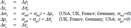
where Δρt, Δηt, Δμt, Δπt, and Δεt are mean-zero stationary processes.
A.4 Hypotheses and Results
In a textbook model of monetary policy, the central bank is the monopoly issuer of ‘high-powered’ or base money, for which the public and the banking system have an assured (and somewhat interest-inelastic) demand. The central bank can use its monopoly power to regulate the terms – a short-term interest rate – on which base money is made available to the system. In a deterministic setting of this type, monetary policy can be described, with indifference, as the setting of the amount of base money available, or as the setting of ‘the’ short-term interest rate through which the central bank regulates the supply of base money. In fact, central bankers often seem to prefer to describe their activities in terms of the setting of ‘the’ interest rate, possibly on the grounds that alternative methods of rationing base money are not often in evidence and because they attach greater value to smoothing interest rates than to smoothing monetary base. However, in general, stochastic analysis of the type introduced by Poole (1970) illustrates the circumstances under which monetary or interest rate targeting might be preferred. As is well known, if the demand for money is relatively unstable, this approach suggests the superiority of taking the interest rate as the immediate target (instrument) of policy; provided that it feeds back on a nominal variable, such a policy need not have the disastrous consequences indicated by Sargent and Wallace (1975). (See McCallum (1981) and Edey (1990)). There is a suggestion in the literature that during the 1980s, the central banking authorities of the developed countries have converged on a view that monetary policy is best conceived of as a matter of setting ‘the’ short-term interest rate with respect to achieving objectives in price and output directly (Batten et al. 1990). In this story monetary aggregates are by-passed. An explanation might be the unsettling experience of the effects of financial liberalisation on the behaviour of the monetary aggregates in some countries. An alternative view is that, in fact, the focus on a narrow set of interest rates unduly restricts the perception of what monetary policy can (and does) do. The monetarist literature of the 1960s is full of suggestions to this effect.
These considerations underlie two of the principal issues to be investigated in the rest of this paper. They are these: is there evidence that money is important for output and prices? And, if so, is that importance fully accounted for by the significance that money has for interest rates and the importance of interest rates for prices and output? These questions can of course also be asked of the data in reverse. That is, we can ask whether interest rates are stably related to output and prices and whether, if so, that relationship can as well or better be accounted for by the effect of interest rates on money, and of money on output and prices.
Descriptions of the transmission mechanism of monetary policy generally go further, to indicate how it is that money and/or interest rates affect prices and/or output. For example, it is often argued that in an open economy, the exchange rate is a major ‘channel of effect’ of monetary policy; whilst some form of Phillips curve remains a standard feature in the transmission of monetary actions, which impact on real output, to prices. The concepts of unconditional and conditional causality can also be brought to bear on these issues.
A.4.1 Money and Interest Rates: Output
Tables A3 to A6 provide the necessary information to analyse the money/interest rate-output relationship. Table A3 gives the unconditional feedback measures for money and output. As can readily be seen, the money-output feedback appears to be highly significant at all but the shortest lag for the United Kingdom, significant at all lags for France, and more weakly for the United States. In the case of Germany, the feedback essentially appears only significant at the longest (12-month and more) lags.[22] ‘Reverse’ causality is prominent and highly significant at all lags for France, and is quite significant for the USA. Instantaneous feedback is present, but mainly only at the 10 per cent level of significance, in the USA, but not elsewhere.
The feedbacks in Table A4 are not so pervasive. Interest rate-output feedbacks are significant at some lag for every country. But in Germany, it is only detectable at the longest (24-month) lag at better than 5 per cent levels of significance. In France, the feedback is significant at such levels only at the 18-month and 24-month lags; in the United Kingdom, the feedback is significant at nearly all lags but not strongly so. In the United States, the feedback is strongly significant at 18 and 24 months, and is significant at the 5 per cent level also at 12 months.
Table A5 then shows that the relationship between interest rates and money – perhaps, not so pervasive as might be supposed. In general, little significant feedback, either from interest rates to money or in the reverse direction, is evident in either the United Kingdom or France, though instantaneous feedback can be found for the United Kingdom at all lags at the 5 per cent level of significance. In Germany and more especially the United States, on the other hand, the feedbacks are by contrast pervasive and strong.
When the money-output and interest rate-output feedbacks are conditioned on the ‘other’ variable, as in Table A6, some interesting results emerge. To start with, for the most surprising case, the United Kingdom, what is revealed is that the powerful money-output feedback is not weakened when conditioned upon the interest rate. In the language of the transmission mechanism, the importance of money for output – which is clear at all lags except the shortest – does not depend upon an interest rate ‘channel of effect’. Indeed, if anything, the opposite is the case. Insofar as the interest rate is important for output, it is through money: for, when the conditional feedback is computed, the significance of the former feedback disappears. The results for France are in a similar mould. Here, also, the money-output feedback is important and its significance is not notably weakened when conditioned on the interest rate.
The results for the United States confirm a more Keynesian view of the transmission mechanism. Here, conditioning the money-output feedback on the interest rate removes its significance, whilst conditioning the interest rate-output feedback on money serves to sustain its significance.
The money-output feedbacks for Germany are somewhat less pervasive than elsewhere; but conditioning on the interest rate does not weaken them.
On this basis, one country in the sample – the United States – exhibits a Keynesian transmission mechanism; but two – the United Kingdom and France – clearly do not, whilst the fourth country, Germany, also falls into the second rather than the first camp.
Do these findings for the transmission mechanism in respect of output apply equally to prices? Tables A7 to A9 provide the relevant evidence on this question.
A.4.2 Money and Interest Rates: Prices
Table A7 shows that it is only for the United Kingdom that a significant money-prices feedback can be detected, although ‘reverse’ causality (prices to money) is present everywhere. Nor is the absence of feedback the consequence of overlooking the presence of a long-run cointegrating relationship – for we have already tested for this (Table A2) and found an absence of bivariate cointegration between money and prices. The UK money-prices feedback, moreover, remains significant when conditioned upon the interest rate (Table A9). Table A8 shows, however, that interest rates are important for prices in every country (in Germany only at the longest lag), including the United Kingdom. Moreover, in Table A9, it appears that when these interest rate-prices feedbacks are conditioned on money, they remain significant (with the striking exception of the United Kingdom).
On this basis then, our conclusion is that the transmission mechanism of monetary policy works through the interest rate for prices (except in the United Kingdom) and through the money supply for output (except in the United States). We do not find any general cases where it is impossible to tell money and interest rates apart, perhaps a somewhat surprising finding.
A.4.3 The Phillips Curve
The results in Table A10 enable us to consider whether money (see Table A8) or interest rates (see Table A9) have their effects on prices ‘through’ the Phillips curve – that is, whether or not the relevant feedback, when conditioned on output, tends to disappear.
In fact, the United Kingdom is the only case where a significant money-prices feedback was detected. The strength and significance of that feedback is not altered by conditioning on output, suggesting on this interpretation that the Phillips curve is not an important part of the transmission process.
In Table A9, however, many instances were reported in which a significant interest rate-prices feedback was detected. Turning then to Table A10, it can be seen that only in the United States is there a strong output-prices feedback; so it is not too surprising to find that for this economy conditioning for the interest rate-prices feedback on output causes the feedback to weaken in significance considerably. The Phillips curve effect is important. For France and the United Kingdom, this same form of conditioning does not remove or significantly change the quite strong interest rate-prices feedbacks to be found in those countries. In the case of Germany, the feedback is much less pervasive to start with.
A.4.4 The Exchange Rate
During the 1980s, many countries discovered the role of the exchange rate in the monetary transmission mechanism. Disinflating through adherence to an external standard rather than through maintaining an internal standard became the norm, especially in Europe. It therefore seemed worthwhile investigating the position of the exchange rate in the transmission mechanism. Tables A11 to A13 illustrate this. The results shown are disappointing. The predominant significant relationship is an instantaneous one involving the interest rate with the exchange rate. There is little evidence of exchange rate effects on output (Table A12) or on inflation (Table A13). The main exceptions are the exchange rate feedback to prices in France, less significantly in Germany and the United States. Also, the role of the exchange rate in the transmission mechanism of monetary policy does not appear to be strong.
It could be argued that the effect of nominal exchange rates on output ought to be expected to be weak and that a real exchange rate would be a more appropriate concept to investigate; and regarding prices, it could be argued that a more appropriate transformation would be (e+p*), the domestic price equivalent of foreign prices. Limitations of time prevent the investigation of these claims. But it is not obvious that it is inappropriate to use the nominal exchange rate given the techniques used here.
A.5 Conclusions
The results obtained provide evidence that the transmission mechanism of monetary policy varies from one country to another in our sample. This may be due in part to our prior selection of particular (and different) monetary magnitudes for study in the different cases. This given, the study provides strong support for the conception of monetary policy as setting interest rates to hit targets for prices directly rather than through money (with the United Kingdom as a prominent exception). On the other hand, we have evidence that money is important for real output; only in the United States is it appropriate to say that this effect is mediated ‘through’ the interest rate. It also appears that it is only in the United States that the Phillips curve is an important part of the transmission of monetary actions (on interest rates) to prices.
The suggestion that in an open economy the exchange rate provides a significant part of the transmission mechanism of monetary policy received little support from the techniques (and data definitions) used here.
Two caveats should be repeated. Firstly, the techniques and interpretations offered appeal essentially to an assumption of causality in the processes concerned. Yet it may be that the evidence we have, for example, of interest rates feeding back to prices at quite long lags is influenced by central bank inflation predictions and reaction functions in setting interest rates. Secondly, the term ‘transmission mechanism’ has been used in a technical way; confronted by our evidence that M0 causes changes in output (and prices) in the United Kingdom in a way that is not significantly connected to the interest rate, central bankers would be likely to argue that this ‘cannot be’ a correct description of their policy, which is to supply M0 ‘on demand’ at the given interest rate. M0 must be a proxy for some other variable that is ‘really doing the work’. This may very well be, but for the moment it is unproven, and may well remain unprovable.[23]
Results
| Unit root tests | t statistics for a regression of ΔX on: | ||||||
|---|---|---|---|---|---|---|---|
| Series | DF(Z)a | DF(Z) | DF(ΔZ)a | DF(ΔZ) | Drift | Time | |
| United States | y | −3.28 | −3.21 | −5.29** | −4.78** | 0.80 | −0.25 |
| m | 0.21 | 0.16 | −4.97** | −4.84** | 4.04** | −2.66** | |
| P | −0.93 | −1.14 | −3.86* | −3.10 | 2.46** | −1.29 | |
| i | −2.33 | −2.11 | −7.47** | −7.35** | 1.02 | −0.91 | |
| e | −1.43 | −1.43 | −5.64** | −4.87** | 0.14 | −0.33 | |
| United Kingdom | y | −2.57 | −2.49 | −7.04** | −6.21** | 0.25 | 0.09 |
| m | −0.54 | −0.68 | −5.45** | −4.09** | 3.61** | −2.57** | |
| P | −0.53 | −1.06 | −4.90** | −3.78* | 2.69** | −1.72* | |
| i | −2.76 | −3.29 | −5.66** | −5.38** | 0.15 | −0.04 | |
| e | −2.09 | −2.16 | −6.77** | −5.90** | −1.40 | 1.06 | |
| France | y | −2.92 | −3.31 | −7.12** | −5.05** | 1.04 | −0.59 |
| m | 0.25 | 0.09 | −5.34** | −4.50** | 3.47** | −3.24** | |
| P | 0.41 | −0.47 | −3.73* | −2.82 | 2.88** | −2.21* | |
| i | −2.56 | −2.55 | −6.16** | −5.33** | 0.22 | −0.17 | |
| e | −2.02 | −1.91 | −5.18** | −5.37** | −0.14 | −0.04 | |
| Germany | y | −2.06 | −2.17 | −6.73** | −5.59** | 0.57 | −0.07 |
| m | −2.18 | −2.24 | −5.41** | −4.51** | 2.71** | −1.36 | |
| P | −0.78 | −0.48 | −6.73** | −5.99** | −5.59** | −4.49** | |
| i | −2.49 | −2.31 | −8.47** | −6.26** | −0.61 | 0.64 | |
| e | −2.30 | −2.20 | −7.19** | −5.68** | −1.71* | −1.04 | |
| Notes: Significant at the 1% level (**) and 5% level (*). All statistics are based on regressions with six lags except (a) which has four lags. DF(Z) and DF(ΔZ) refer to the Dickey-Fuller t statistic computed for the level (Z) and the first difference (ΔZ) in a regression including a constant and a time trend (Fuller 1976, p. 373). | |||||||
| System | United States | Engle-Yoo (Z) | Germany | |
|---|---|---|---|---|
| United Kingdom | France | |||
| y = α0 + α1i | −0.66 | −1.31 | −1.43 | −0.30 |
| y = α0 + α1m | −3.01 | −2.08 | −0.60 | −2.14 |
| y = α0 + α1i | −0.67 | −1.49 | −1.97 | −0.39 |
| y = α0 + α1m + α2i | −2.86 | −2.15 | −0.59 | −2.13 |
| p = α0 + α1i | −0.75 | −1.41 | −0.76 | −1.09 |
| p = α0 + α1m | −1.91 | −2.33 | −0.95 | −1.71 |
| p = α0 + α1m + α2i | −2.49 | −2.28 | −1.73 | −1.39 |
| p = α0 + α1y | −2.50 | −1.78 | −2.14 | −1.82 |
| e = α0 + α1i | −1.45 | −1.77 | −0.99 | −1.28 |
| Note: Engle-Yoo refers to the Engle-Yoo (1987) Augmented Dickey-Fuller tests with four lags. | ||||
| Feedback | Measure of linear feedback (lag, number of months) |
||||||
|---|---|---|---|---|---|---|---|
| 24 | 18 | 12 | 9 | 6 | 3 | ||
| United States | Δm → Δy | 0.150+ | 0.142* | 0.103* | 0.096* | 0.092** | 0.058** |
| Δy → Δm | 0.207** | 0.142* | 0.089+ | 0.081* | 0.067* | 0.053** | |
| Δm – Δy | 0.016+ | 0.016+ | 0.018* | 0.017+ | 0.017+ | ||
| United Kingdom | Δm → Δy | 0.253** | 0.199** | 0.134** | 0.127** | 0.077** | 0.008 |
| Δy → Δm | 0.115 | 0.084 | 0.039 | 0.037 | 0.035 | 0.005 | |
| Δm – Δy | 0.003 | 0.009 | 0.007 | 0.007 | 0.005 | ||
| France | Δm → Δy | 0.400** | 0.289** | 0.235* | 0.222** | 0.168** | 0.160** |
| Δy → Δm | 0.416** | 0.372** | 0.308** | 0.267** | 0.228** | 0.146** | |
| Δm – Δy | 0.000 | 0.001 | 0.003 | 0.004 | 0.005 | ||
| Germany | Δm → Δy | 0.225** | 0.205** | 0.110* | 0.059 | 0.053+ | 0.007 |
| Δy → Δm | 0.144 | 0.102 | 0.083 | 0.074+ | 0.038 | 0.005 | |
| Δm – Δy | 0.003 | 0.002 | 0.003 | 0.005 | 0.006 | ||
| Notes: (a) Significant at the 1% level (**); 5% level (*) and 10% level
(+). (b) ‘→’ indicates feedback from left-hand side variable to right-hand side variable. (c) ‘–’ indicates instantaneous feedback between left-hand side variable and right-hand side variable. |
|||||||
| Feedback | Measure of linear feedback (lag, number of months) |
||||||
|---|---|---|---|---|---|---|---|
| 24 | 18 | 12 | 9 | 6 | 3 | ||
| United States | Δi → Δy | 0.225** | 0.160** | 0.116* | 0.073+ | 0.040 | 0.026 |
| Δy → Δi | 0.280** | 0.262** | 0.226** | 0.184** | 0.163** | 0.157** | |
| Δi – Δy | 0.114** | 0.108** | 0.109** | 0.104** | 0.083** | ||
| United Kingdom | Δi → Δy | 0.161+ | 0.137* | 0.090+ | 0.77* | 0.049+ | 0.006 |
| Δy → Δi | 0.089 | 0.075 | 0.060 | 0.036 | 0.021 | 0.005 | |
| Δi – Δy | 0.008 | 0.008 | 0.010 | 0.009 | 0.005 | ||
| France | Δi → Δy | 0.211** | 0.149* | 0.058 | 0.031 | 0.024 | 0.016 |
| Δy → Δi | 0.129 | 0.094 | 0.075 | 0.063 | 0.056+ | 0.014 | |
| Δi – Δy | 0.001 | 0.001 | 0.001 | 0.001 | 0.001 | ||
| Germany | Δi → Δy | 0.217** | 0.087 | 0.048 | 0.047 | 0.039 | 0.029+ |
| Δy → Δi | 0.106 | 0.091 | 0.078 | 0.076* | 0.059* | 0.021 | |
| Δi – Δy | 0.000 | 0.001 | 0.001 | 0.000 | 0.001 | ||
| Notes: (a) Significant at the 1% level (**); 5% level (*) and 10% level
(+). (b) ‘→’ indicates feedback from left-hand side variable to right-hand side variable. (c) ‘–’ indicates instantaneous feedback between left-hand side variable and right-hand side variable. |
|||||||
| Feedback | Measure of linear feedback (lag, number of months) |
||||||
|---|---|---|---|---|---|---|---|
| 24 | 18 | 12 | 9 | 6 | 3 | ||
| United States | Δm → Δi | 0.146 | 0.119+ | 0.095* | 0.088* | 0.082** | 0.055** |
| Δi → Δm | 0.361** | 0.330** | 0.298** | 0.284** | 0.262** | 0.190** | |
| Δm – Δi | 0.034** | 0.028* | 0.026** | 0.027* | 0.025* | ||
| United Kingdom | Δm → Δi | 0.137 | 0.088 | 0.074 | 0.070+ | 0.060* | 0.050* |
| Δi → Δm | 0.150+ | 0.101 | 0.066 | 0.033 | 0.015 | 0.009 | |
| Δm – Δi | 0.012 | 0.021* | 0.023* | 0.023* | 0.021* | ||
| France | Δm → Δi | 0.306* | 0.257* | 0.097 | 0.052 | 0.016 | 0.011 |
| Δi → Δm | 0.240 | 0.158 | 0.115 | 0.055 | 0.053 | 0.007 | |
| Δm – Δi | 0.017 | 0.017 | 0.016 | 0.018 | 0.012 | ||
| Germany | Δm → Δi | 0.226** | 0.161** | 0.090+ | 0.086* | 0.080** | 0.054** |
| Δi → Δm | 0.446** | 0.323** | 0.290** | 0.249** | 0.229** | 0.218** | |
| Δm – Δi | 0.020* | 0.018* | 0.015+ | 0.011 | 0.008 | ||
| Notes: (a) Significant at the 1% level (**); 5% level (*) and 10% level
(+). (b) ‘→’ indicates feedback from left-hand side variable to right-hand side variable. (c) ‘–’ indicates instantaneous feedback between left-hand side variable and right-hand side variable. |
|||||||
| Feedback | Measure of linear feedback (lag, number of months) |
||||||
|---|---|---|---|---|---|---|---|
| 24 | 18 | 12 | 9 | 6 | 3 | ||
| United States | Δm → Δy | 0.150+ | 0.142* | 0.103* | 0.096* | 0.092** | 0.058** |
| Δm → Δy/Δi | 0.093 | 0.081 | 0.059 | 0.051 | 0.044 | 0.017 | |
| Δi → Δy | 0.225** | 0.160** | 0.116* | 0.073* | 0.040 | 0.026 | |
| Δi → Δy/Δm | 0.176* | 0.099 | 0.061 | 0.041 | 0.015 | 0.005 | |
| Δm · Δi → Δy | 0.338** | 0.241* | 0.167* | 0.126+ | 0.103* | 0.065* | |
| United Kingdom | Δm → Δy | 0.253** | 0.199** | 0.134** | 0.127** | 0.077** | 0.008 |
| Δm → Δy/Δi | 0.228** | 0.189** | 0.128** | 0.124** | 0.058* | 0.001 | |
| Δi → Δy | 0.161* | 0.137* | 0.090+ | 0.077* | 0.049+ | 0.006 | |
| Δi → Δy/Δm | 0.147 | 0.128+ | 0.068 | 0.062 | 0.033 | 0.013 | |
| Δm · Δi → Δy | 0.390** | 0.327** | 0.203** | 0.189** | 0.114** | 0.013 | |
| France | Δm → Δy | 0.400** | 0.289** | 0.235* | 0.222** | 0.168** | 0.160** |
| Δm → Δy/Δi | 0.472** | 0.358** | 0.264** | 0.233** | 0.157** | 0.143** | |
| Δi → Δy | 0.211** | 0.149* | 0.058 | 0.031 | 0.024 | 0.016 | |
| Δi → Δy/Δm | 0.448** | 0.336** | 0.078 | 0.045 | 0.038 | 0.014 | |
| Δm · Δi → Δy | 0.916** | 0.625** | 0.321* | 0.274* | 0.193* | 0.165** | |
| Germany | Δm → Δy | 0.225** | 0.205** | 0.110* | 0.059 | 0.053+ | 0.007 |
| Δm → Δy/Δi | 0.282** | 0.264** | 0.100* | 0.045 | 0.036 | 0.002 | |
| Δi → Δy | 0.217** | 0.087 | 0.048 | 0.047 | 0.039 | 0.029 | |
| Δi → Δy/Δm | 0.221** | 0.146** | 0.043 | 0.040 | 0.027 | 0.020 | |
| Δm · Δi → Δy | 0.453** | 0.351** | 0.159+ | 0.100 | 0.079 | 0.032 | |
| Notes: (a) Significant at the 1 % level (**); 5% level (*) and 10% level
(+). (b) ‘→’ indicates feedback from left-hand side variables to right-hand side variables. (c) ‘–’ indicates feedback from left-hand side variable to right-hand side variables conditional on right-hand side variables. |
|||||||
| Feedback | Measure of linear feedback (lag, number of months) |
||||||
|---|---|---|---|---|---|---|---|
| 24 | 18 | 12 | 9 | 6 | 3 | ||
| United States | Δm → Δp | 0.096 | 0.058 | 0.042 | 0.033 | 0.026 | 0.018 |
| Δp → Δm | 0.235** | 0.209** | 0.128** | 0.106** | 0.049+ | 0.036* | |
| Δp – Δm | 0.007 | 0.007 | 0.012* | 0.014+ | 0.011 | ||
| United Kingdom | Δm → Δp | 0.213** | 0.181** | 0.138** | 0.129** | 0.093** | 0.021 |
| Δp → Δm | 0.173* | 0.148* | 0.105* | 0.053 | 0.045 | 0.022 | |
| Δp – Δm | 0.000 | 0.000 | 0.000 | 0.000 | 0.000 | ||
| France | Δm → Δp | 0.209 | 0.119 | 0.087 | 0.022 | 0.013 | 0.003 |
| Δp → Δm | 0.273+ | 0.212 | 0.176* | 0.141* | 0.119* | 0.050 | |
| Δp – Δm | 0.014 | 0.005 | 0.010 | 0.010 | 0.011 | ||
| Germany | Δm → Δp | 0.108 | 0.083 | 0.061 | 0.019 | 0.007 | 0.005 |
| Δp → Δm | 0.207** | 0.184** | 0.137** | 0.065 | 0.065* | 0.021 | |
| Δp – Δm | 0.005 | 0.003 | 0.004 | 0.005 | 0.002 | 0.003 | |
| Notes: (a) Significant at the 1% level (**); 5% level (*) and 10% level
(+). (b) ‘→’ indicates feedback from left-hand side variable to right-hand side variable. (c) ‘–’ indicates instantaneous feedback between left-hand side variable and right-hand side variable. |
|||||||
| Feedback | Measure of linear feedback (lag, number of months) |
||||||
|---|---|---|---|---|---|---|---|
| 24 | 18 | 12 | 9 | 6 | 3 | ||
| United States | Δi → Δp | 0.239** | 0.193** | 0.174** | 0.157** | 0.123** | 0.113** |
| Δp → Δi | 0.102 | 0.092 | 0.075 | 0.058 | 0.046 | 0.027 | |
| Δi – Δp | 0.001 | 0.001 | 0.000 | 0.000 | 0.000 | ||
| United Kingdom | Δi → Δp | 0.263** | 0.166** | 0.113* | 0.099** | 0.092** | 0.063** |
| Δp → Δi | 0.116 | 0.069 | 0.055 | 0.040 | 0.025 | 0.022 | |
| Δi – Δp | 0.001 | 0.000 | 0.000 | 0.000 | 0.000 | ||
| France | Δi → Δp | 0.235** | 0.171** | 0.100* | 0.094* | 0.071* | 0.035+ |
| Δp → Δi | 0.219** | 0.173** | 0.135** | 0.102** | 0.096** | 0.014 | |
| Δi – Δp | 0.031** | 0.027* | 0.028* | 0.026* | 0.026* | ||
| Germany | Δi → Δp | 0.177** | 0.127+ | 0.070 | 0.054 | 0.048 | .017 |
| Δp → Δi | 0.220** | 0.172** | 0.100* | 0.084* | 0.073* | 0.016 | |
| Δi – Δp | 0.028* | 0.018* | 0.018* | 0.018* | 0.017+ | ||
| Notes: (a) Significant at the 1% level (**); 5% level (*) and 10% level
(+). (b) ‘→’ indicates feedback from left-hand side variable to right-hand side variable. (c) ‘–’ indicates instantaneous feedback between left-hand side variable and right-hand side variable. |
|||||||
| Feedback | Measure of linear feedback (lag, number of months) |
||||||
|---|---|---|---|---|---|---|---|
| 24 | 18 | 12 | 9 | 6 | 3 | ||
| United States | Δm → Δp | 0.096 | 0.058 | 0.042 | 0.033 | 0.026 | 0.013 |
| Δm → Δp/Δi | 0.119 | 0.109 | 0.061 | 0.047 | 0.032 | 0.016 | |
| Δi → Δp | 0.239** | 0.193** | 0.174** | 0.157** | 0.123** | 0.113** | |
| Δi → Δp/Δm | 0.234** | 0.244** | 0.217** | 0.158** | 0.128** | 0.109** | |
| Δm.Δi → Δp | 0.351** | 0.302** | 0.224** | 0.184** | 0.137** | 0.121** | |
| United Kingdom | Δm → Δp | 0.213** | 0.181** | 0.138** | 0.129** | 0.093** | 0.021 |
| Δm → Δp/Δi | 0.202** | 0.164** | 0.118** | 0.114** | 0.062* | 0.012 | |
| Δi → Δp | 0.263** | 0.166** | 0.113* | 0.099** | 0.092** | 0.063** | |
| Δi → Δp/Δm | 0.249** | 0.149* | 0.093+ | 0.077* | 0.060* | 0.046* | |
| Δm.Δi → Δp | 0.407** | 0.300** | 0.200** | 0.186** | 0.136** | 0.024 | |
| France | Δm → Δp | 0.209 | 0.119 | 0.087 | 0.022 | 0.013 | 0.003 |
| Δm → Δp/Δi | 0.365** | 0.241* | 0.127 | 0.035 | 0.028 | 0.017 | |
| Δi → Δp | 0.235** | 0.171** | 0.100* | 0.094* | 0.071* | 0.035+ | |
| Δi → Δp/Δm | 0.636** | 0.602** | 0.280** | 0.277** | 0.139** | 0.109** | |
| Δm.Δi → Δp | 0.863** | 0.720** | 0.349* | 0.229+ | 0.114 | 0.087 | |
| Germany | Δm → Δp | 0.108 | 0.083 | 0.061 | 0.019 | 0.007 | 0.005 |
| Δm → Δp/Δi | 0.116 | 0.092 | 0.074 | 0.018 | 0.004 | 0.004 | |
| Δi → Δp | 0.177** | 0.127+ | 0.070 | 0.054 | 0.048 | 0.017 | |
| Δi → Δp/Δm | 0.184* | 0.136* | 0.082 | 0.057 | 0.049+ | 0.020 | |
| Δm.Δi → Δp | 0.292+ | 0.219+ | 0.135 | 0.073 | 0.054 | 0.019 | |
| Notes: (a) Significant at the 1% level (**); 5% level (*) and 10% level
(+). (b) ‘→’ indicates feedback from left-hand side variables to right-hand side variables. (c) ‘·’ indicates feedback from left-hand side variables to right-hand side variables conditional on right-hand side variables. |
|||||||
| Feedback | Measure of linear feedback (lag, number of months) |
||||||
|---|---|---|---|---|---|---|---|
| 24 | 18 | 12 | 9 | 6 | 3 | ||
| United States | Δp → Δy | 0.116 | 0.099 | 0.085+ | 0.066+ | 0.055+ | 0.041* |
| Δy → Δp | 0.183* | 0.135* | 0.118** | 0.098** | 0.068* | 0.068** | |
| Δm → Δp/Δy | 0.107 | 0.072 | 0.030 | 0.017 | 0.010 | 0.008 | |
| Δm.Δy → Δp | 0.302* | 0.207 | 0.153+ | 0.115 | 0.082 | 0.079** | |
| Δi → Δp | 0.239** | 0.193** | 0.174** | 0.157** | 0.123** | 0.113** | |
| Δi → Δp/Δy | 0.185* | 0.132* | 0.109* | 0.094* | 0.051+ | 0.037* | |
| Δi.Δy → Δp | 0.379** | 0.267** | 0.238** | 0.206** | 0.139** | 0.127** | |
| United Kingdom | Δp → Δy | 0.213** | 0.176** | 0.110* | 0.100** | 0.071* | 0.067** |
| Δy → Δp | 0.177* | 0.115 | 0.075 | 0.056 | 0.036 | 0.003 | |
| Δm → Δp/Δy | 0.224** | 0.185** | 0.133** | 0.129** | 0.114** | 0.033+ | |
| Δm.Δy → Δp | 0.407** | 0.300** | 0.200** | 0.186** | 0.136** | 0.024 | |
| Δi → Δp | 0.263** | 0.166** | 0.113* | 0.099** | 0.092** | 0.063** | |
| Δi → Δp/Δy | 0.324** | 0.232** | 0.177** | 0.129** | 0.112** | 0.086** | |
| Δi.Δy → Δp | 0.485** | 0.346** | 0.226** | 0.160** | 0.128** | 0.073* | |
| France | Δp → Δy | 0.180* | 0.105 | 0.064 | 0.059 | 0.032 | 0.026 |
| Δy → Δp | 0.147 | 0.127+ | 0.087+ | 0.085* | 0.067* | 0.039* | |
| Δm → Δp/Δy | 0.361** | 0.200 | 0.060 | 0.013 | 0.011 | 0.011 | |
| Δm.Δy → Δp | 0.693** | 0.377 | 0.190 | 0.119 | 0.080 | 0.020 | |
| Δi → Δp | 0.235** | 0.171** | 0.100* | 0.094* | 0.071* | 0.035+ | |
| Δi → Δp/Δy | 0.210** | 0.152* | 0.102* | 0.098* | 0.080** | 0.049* | |
| Δi.Δy → Δp | 0.370** | 0.291** | 0.190** | 0.141** | 0.128** | 0.084** | |
| Germany | Δp → Δy | 0.175* | 0.142* | 0.109* | 0.070+ | 0.067* | 0.055** |
| Δy → Δp | 0.164+ | 0.115 | 0.090+ | 0.049 | 0.026 | 0.020 | |
| Δm → Δp/Δy | 0.136 | 0.103 | 0.072 | 0.023 | 0.019 | 0.016 | |
| Δm.Δy → Δp | 0.314* | 0.218+ | 0.149* | 0.067+ | 0.024* | 0.024** | |
| Δi → Δp | 0.177* | 0.127+ | 0.070 | 0.054 | 0.048 | 0.017 | |
| Δi → Δp/Δy | 0.182* | 0.131+ | 0.090+ | 0.068+ | 0.061* | 0.018 | |
| Δi.Δy → Δp | 0.361** | 0.275* | 0.184* | 0.106 | 0.074 | 0.038 | |
| Notes: (a) Significant at the 1% level (**); 5% level (*) and 10% level
(+). (b) ‘→’ indicates feedback from left-hand side variables to right-hand side variables. (c) ‘·’ indicates feedback from left-hand side variable to right-hand side variables conditional on right-hand side variables. |
|||||||
| Feedback | Measure of linear feedback (lag, number of months) |
||||||
|---|---|---|---|---|---|---|---|
| 24 | 18 | 12 | 9 | 6 | 3 | ||
| United States | Δi → Δe | 0.123 | 0.093 | 0.061 | 0.055 | 0.040 | 0.024 |
| Δe → Δi | 0.126 | 0.089 | 0.055 | 0.044 | 0.037 | 0.026 | |
| Δi – Δe | 0.023* | 0.024* | 0.030** | 0.031** | 0.034** | ||
| United Kingdom | Δi → Δe | 0.137 | 0.120+ | 0.055 | 0.044 | 0.038 | 0.031+ |
| Δe → Δi | 0.158+ | 0.120+ | 0.094* | 0.066+ | 0.052+ | 0.037* | |
| Δi – Δe | 0.185** | 0.171** | 0.135** | 0.142** | 0.143** | ||
| France | Δi → Δe | 0.240** | 0.169** | 0.071 | 0.053 | 0.035 | 0.017 |
| Δe → Δi | 0.129 | 0.083 | 0.064 | 0.039 | 0.030 | 0.006 | |
| Δi – Δe | 0.043** | 0.044** | 0.040** | 0.034** | 0.033** | ||
| Germany | Δi → Δe | 0.231** | 0.122+ | 0.066 | 0.059 | 0.029 | 0.020 |
| Δi → Δe | 0.158+ | 0.135* | 0.113* | 0.090* | 0.044 | 0.039* | |
| Δi – Δe | 0.003 | 0.003 | 0.001 | 0.001 | 0.000 | ||
| Notes: (a) Significant at the 1% level (**); 5% level (*) and 10% level
(+). (b) ‘→’ indicates feedback from left-hand side variable to right-hand side variable. (c) ‘–’ indicates instantaneous feedback between left-hand side variable and right-hand side variable. |
|||||||
| Feedback | Measure of linear feedback (lag, number of months) |
||||||
|---|---|---|---|---|---|---|---|
| 24 | 18 | 12 | 9 | 6 | 3 | ||
| United States | Δy → Δe | 0.053 | 0.041 | 0.029 | 0.018 | 0.016 | 0.009 |
| Δe → Δy | 0.125 | 0.091 | 0.065 | 0.038 | 0.034 | 0.021 | |
| Δy – Δe | 0.019* | 0.023* | 0.024* | 0.028* | 0.029* | ||
| United Kingdom | Δy → Δe | 0.151+ | 0.119+ | 0.093+ | 0.041 | 0.035 | 0.009 |
| Δe → Δy | 0.109 | 0.090 | 0.066 | 0.057 | 0.044 | 0.038* | |
| Δy – Δe | 0.000 | 0.000 | 0.000 | 0.001 | 0.000 | ||
| France | Δy → Δe | 0.178* | 0.100 | 0.066 | 0.058 | 0.022 | 0.013 |
| Δe → Δy | 0.220** | 0.196** | 0.134** | 0.068+ | 0.017 | 0.014 | |
| Δy – Δe | 0.003 | 0.006 | 0.005 | 0.005 | 0.005 | ||
| Germany | Δy → Δe | 0.120 | 0.101 | 0.079 | 0.069+ | 0.046 | 0.029* |
| Δe → Δy | 0.081 | 0.068 | 0.031 | 0.021 | 0.020 | 0.007 | |
| Δy – Δe | 0.024* | 0.023* | 0.024* | 0.023* | 0.020* | ||
| Notes: (a) Significant at the 1% level (**); 5% level (*) and 10% level
(+). (b) ‘→’ indicates feedback from left-hand side variable to right-hand side variable. (c) ‘–’ indicates instantaneous feedback between left-hand side variable and right-hand side variable. |
|||||||
| Feedback | Measure of linear feedback (lag, number of months) |
||||||
|---|---|---|---|---|---|---|---|
| 24 | 18 | 12 | 9 | 6 | 3 | ||
| United States | Δp → Δe | 0.163* | 0.155* | 0.103* | 0.088* | 0.064 | .007 |
| Δe → Δp | 0.150+ | 0.121+ | 0.101* | 0.084* | 0.066* | 0.029+ | |
| Δp – Δe | 0.009 | 0.009 | 0.005 | 0.006 | 0.010 | ||
| United Kingdom | Δp → Δe | 0.135 | 0.108 | 0.027 | 0.016 | 0.012 | 0.011 |
| Δe → Δp | 0.078 | 0.064 | 0.019 | 0.009 | 0.006 | 0.002 | |
| Δp – Δe | 0.002 | 0.002 | 0.003 | 0.003 | 0.003 | ||
| France | Δp → Δe | 0.181* | 0.137* | 0.050 | 0.038 | 0.027 | 0.019 |
| Δe → Δp | 0.195* | 0.153* | 0.099** | 0.079* | 0.034 | 0.012 | |
| Δp – Δe | 0.002 | 0.002 | 0.004 | 0.005 | 0.003 | ||
| Germany | Δp → Δe | 0.109 | 0.084 | 0.043 | 0.036 | 0.018 | 0.013 |
| Δe → Δp | 0.141 | 0.103 | 0.084 | 0.082* | 0.066* | 0.040* | |
| Δp – Δe | 0.002 | 0.000 | 0.000 | 0.000 | 0.000 | ||
| Notes: (a) Significant at the 1% level (**); 5% level (*) and 10% level
(+). (b) ‘→’ indicates feedback from left-hand side variable to right-hand side variable. (c) ‘–’ indicates instantaneous feedback between left-hand side variable and right-hand side variable. |
|||||||
Appendix B: The Wage-Price Mark-Up Model
The most basic building block in the view that the exchange rate matters for prices is the traditional mark-up model. This gives prices as a mark-up over costs – in an open economy, wage costs and import costs. The mark-up may vary with demand. Wage costs can also be represented as a mark-up over prices (see the Layard-Nickell (1985) view of inflation as ‘a battle of the mark-ups’) and this mark-up may also vary with the state of demand.
This set up delivers the following important propositions:
- starting from a given state of demand, a nominal devaluation of x per cent produces a rise in prices and wages of x per cent. Real wages and the real exchange rate are unaffected.
- this is true no matter how small the importance of import costs in the price index.
- in practice there are lags in the adjustment of wages to prices and of prices to costs. For this reason, a nominal devaluation will immediately produce a real devaluation which will wear off over time as prices and wages adjust.
- allowing for demand to change in the experiment, a nominal devaluation will lead initially to a real devaluation and so to some increase in demand. The demand increase will raise mark-ups and may produce a period of real exchange rate appreciation. The length of the adjustment period will be increased.
- all the above is straightforward as an analysis of the responses to a nominal devaluation starting from equilibrium. The implicit ‘cause’ of such a devaluation is therefore a monetary shock. The nominal devaluation is unnecessary on any real grounds and the price rises (‘inflation’) that ensue reflect the nature of the shock.
- a real shock would change the equilibrium. Consider a shock which is associated with a devaluation of the equilibrium real exchange rate. This adjustment could be achieved by keeping the exchange rate fixed and allowing domestic wages and prices to fall under the prompting of unemployment and demand declines. As we would be inclined to assume that prices and wages are sticky downwards, it seems that adjustment would be easier if there were a nominal exchange rate devaluation. In this event, an absolute decline in wages and prices need not be called for while adjustment in real wages and the real exchange rate takes place.
- compared with the alternative (fixed nominal exchange rate), nominal devaluation in this case is still ‘inflationary’ (price rises are needed to facilitate real declines), but it is not inflationary in the sense involved in the case of a money shock. Real wages and the real exchange rate fall, rather than remaining constant, and the price rises purchase a reduction in the sacrifice ratio, rather than nothing.
- when demand falls and mark-ups decrease, price and wages ceteris paribus decline. Is the devaluation-wage-price pass through then reduced? Politicians in the ‘outer fringe’ of erstwhile ERM devaluers would like to think so. The algebra says not. There is a demand effect which is depressing margins and reducing prices (and wages). But the devaluation will raise prices and wages in the normal way; in fact, in so far as the devaluation raises demand it will tend to reverse the demand effect, and so will raise prices more than normally. However, to the extent that what is happening is a realisation of the real devaluation scenario described above, we might agree to the politicians' use of language.
- below, to complete the account, we append two items. One is a note of the result of interrogating UK macroeconometric models with the question ‘How big is the effect of a nominal devaluation on prices and wages and how long does it take?’ The second, included at some risk of being obvious, is a reduced form algebraic model borrowed from the European Commission's (EC) Report ‘One Market, One Money’. This is a convenient representation of the mark-up approach.
B.1 Macroeconometric Estimates of the Exchange Rate-Wage-Price Pass-Through
The table below (drawn from Artis and Currie (1981)) logs the effect of a ceteris paribus 5 per cent nominal appreciation on prices and competitiveness in three United Kingdom macroeconometric models, those of H.M. Treasury (HMT), the National Institute of Economic and Social Research (NIESR) and the London Business School (represented by the Beenstock-Burns version). By year five much of the initial effect has been eaten up.[24]
| Model: | Wholesale Prices | Competitiveness(a) | |||||
|---|---|---|---|---|---|---|---|
| HMT | BB | NIESR | HMT | BB | NIESR | ||
| Year | 1 | −0.9 | −2.0 | −1.1 | −1.7 | −3.0 | −3.3 |
| 2 | −1.7 | −2.9 | −2.0 | −1.7 | −1.9 | −1.6 | |
| 3 | −2.6 | −3.6 | −3.2 | −1.2 | −1.2 | −1.3 | |
| 4 | −3.1 | −4.3 | −3.5 | −0.9 | −0.4 | −0.9 | |
| 5 | −3.6 | −4.9 | −3.8 | −0.7 | −0.2 | −0.6 | |
| Note: (a) Relative export prices. | |||||||
B.2 The European Commission Model
The model is representative of the wage-price block of a modern macroeconometric model, and is expressed as follows:
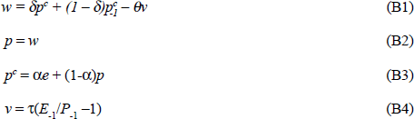
The lower case letters represent rates of growth (Δln). Equation (B1) gives wages as a mark-up on consumer prices with rudimentary dynamics; the mark-up is a function of demand, v. Equation (B2) identifies domestic producer prices with wages (no mark-up) and equation (B3) gives consumer prices in terms of foreign prices (the exchange rate, e) and domestic prices. The demand variations of interest in this context are those due to variations in the real exchange rate, so v is specialised to represent this in (B4).
It is obvious that, for a given level of demand (v=0), an x per cent change in E (e=x), must produce a corresponding increase in w, p and pc. Over the transition path, variations in E/P may in fact occur, affecting the path through v.
Two illustrative simulations of the model are shown in Figures B1 and B2. Figure B1 shows the adjustment of the model to a nominal 10 per cent devaluation on two alternative assumptions about the openness of the economy, as measured by the parameter α. In the highly open economy, α is set at 0.8; in the moderately open economy it is set at 0.2. The other parameters are set as follows: θ = 0.3; τ = 0.07; and δ = 0.5. The initial values of E, P and E/P (the real exchange rate) are normalised to unity. The nominal devaluation is administered by shocking E by 10 per cent. The Figure B1 shows very clearly, that whether the economy is highly or only moderately open, the nominal devaluation initially forces a real devaluation. But, as prices subsequently rise, this is unwound and prices adjust to a level 10 per cent higher than before (right-hand scale) while the real exchange rate declines to its original value of unity (left-hand scale). In the very open economy, however, the adjustment is much faster. The initial adjustment of the real rate is much smaller and is unwound much more quickly. The proposition that the benefit of being able to change the exchange rate peg declines with openness (for example, Krugman (1990)) is illustrated here.
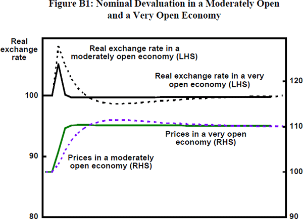
Figure B2 illustrates the case of a real exchange rate shock. The shock is administered by altering the equilibrium value of the real exchange rate by 10 per cent. Two cases are then considered, one in which the real shock is accompanied by a nominal devaluation of the same amount, another in which the nominal rate is held steady. The long-run result in the first case is that prices (right-hand scale) end up at the same level as they hold at the beginning, with initial inflation followed by deflation. The nominal exchange rate depreciates by 10 per cent as does the real exchange rate. In the alternative simulation the whole of the real exchange rate depreciation is accompanied by a fall in the price level. In the model as simulated there is no asymmetry between price level increases and declines, so downward stickiness is not represented. It is easy to see that if downward stickiness were to be represented, this would rule out, or make very expensive, the adjustment via price level alone. In the limit (if downward price adjustments are treated as infeasible), the real exchange rate shock can only be accommodated by nominal devaluation(s).
Appendix C: The Walters Critique
The system discussed in the text can be set out more formally as below:
The additional equation (C6) here serves to describe some possibilities for the nominal interest rate. If β = 0, the ‘Walters case’ holds as interest rates are fully convergent on German levels. A rise in relative inflation would reduce the real rate of interest below German levels. With β = 1, the real rate would be the same as in Germany, with β > 1, the real interest rate rises with the inflation differential.
The system described by equation (C1) – (C6) has the solution in matrix form:

where 
The determinant and trace of the square matrix determine stability (Beavis and Dobbs 1990). Denoting the matrix as A, the values of these are:
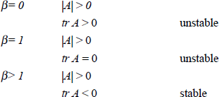
Thus only when the real interest rate rises with inflation (β> 1) is the system stable.
Footnotes
This distinction, between real exchange targeting and nominal exchange rate targeting, is also drawn by two of the authors Williamson (1993) and Corden (1993) in the recent Economic Journal symposium on the subject. [1]
The ‘hard landing’ scenario was described in detail by Marris (1985) who has subsequently argued that part of his purpose in doing so was to lend force to the call for the kind of cooperation that ensued with the Plaza process (Marris 1991). [2]
This is in contrast with the concluding remarks in that volume by Paul Krugman who notes inter alia that: ‘The general verdict, then, must be that the international adjustment process has worked, in both meaningful senses: that is, it has worked acceptably, and it has worked about the way conventional wisdom thought it would’. This comment implies that the literature on ‘pricing to market’ and hysteresis effects, to which Krugman himself subscribed (Baldwin and Krugman 1989), may have less to contribute to an understanding of the adjustment process in the 1980s than appeared at first sight. [3]
To the extent that the intervention works because it is a signal of future monetary policy it is not going to be a complete substitute for such policy. If the signalling is to be credible, it will have to be followed up by the actions that it foreshadows. [4]
The policy was in effect for nearly a year – from March 1987 to January 1988. The first set of bands shown on Figure 3 take the unofficial ceiling of 3DM to the pound sterling and show the central parity and lower limit that would be implied by a ‘narrow band’ ERM membership. The second set of bands, for comparison, shows the position during the period of formal ERM membership, with 6 per cent bands. [5]
It is not correct, however, to place all of the blame on monetary policy (i.e. the decision to target the exchange rate), as fiscal policy could have been used to keep down demand; but it was not. [6]
Actually, the position is a little more complicated than this. XX is a schedule of external balance (constant current account balance) so it is deviations of the economy from this schedule which involve different debt service obligations and so give rise to hysteresis. See Artis and Taylor (1993a). [7]
In recognition of the normative character of the FEER, Artis and Taylor (1993a) have redescribed it as the DEER, or ‘desired equilibrium exchange rate’. [8]
As far as I know, this diagram was first presented by Walter Eltis, then Director of the National Economic Development Office, to explain Chancellor Lawson's policy stance in the period before the episode of shadowing the DM. [9]
Alternatively viewed, this is a natural rate assumption with some inertia in prices and wages. See Appendix B. [10]
Because the ECU itself is a composite currency, the amount by which a country's ECU rate changes before causing the divergence indicator to ‘flash’ depends on the weight of the currency itself in the ECU. [11]
Realignments afforded a further kind of ‘opt-out’. Whilst the ‘German leadership hypothesis’ is the accepted view of the way in which the EMS worked and is supported empirically by studies like that of McDonald and Taylor (1991), there are critics, notably Fratianni and von Hagen (1992). McKinnon (1993) affords a neat contrast of the ‘rules of the EMS game’ as in the ‘Spirit of the Treaty’ and as practised in the Greater Deutschemark Area. [12]
With the exception of the Italian adjustment referred to above. [13]
There is absolutely no published record that the Bundesbank did other than carry out its intervention obligations to the letter. Analysts of the Italian case in particular, however, have drawn attention to the ‘signals’ sent out by Chancellor Kohl's visit to the Bundesbank on 11 September. [14]
The trade-off is particularly sharp when, as appears to be the case for the United Kingdom, the economy is substantially a ‘floating rate economy’ where debt contracts are commonly determined at a variable interest rate. [15]
The credibility bands are computed by assuming that the maximum exchange rate depreciation/appreciation is represented by the official ceiling and floor around the ERM central parity against the DM. Notice that, strictly speaking, because the ERM commitment is multi-bilateral, it was not always the DM that appeared to be proximately the hardest currency. [16]
As Figure 10 shows, interest rates fell during 1991–92 before the crash, but unemployment rose, so that ‘domestically desired’ interest rates were in effect falling faster than actual rates. [17]
These issues have been raised by the International Monetary Fund (IMF) in its World Economic Outlook for May 1993. [18]
Of course, it is always possible that subsets of the variables of interest would cointegrate in the presence of additional, unexplored, variables not included in the data set. [19]
The original study employed only one measure of money in the Italian case whereas three measures were examined in each of the other cases. [20]
Cointegration tests on the exchange rate were limited in view of the unfavourable evidence obtained. [21]
Stock and Watson (1989) found that de-trending money growth revealed stronger money-output links than were apparent otherwise. Krol and Ohanian (1990), however, found that this effect was US-specific and was not a feature of data for other countries in their sample. [22]
For the case in question, supplementary regressions were run conditioning on retail sales data, on the grounds that retail sales might be the key demand variable which is ‘really doing the work’. The conditioning was however completely unsuccessful, leaving the strong and significant leads of money over prices and output intact. [23]
The models concerned represent the early 1980s ‘state of the art’. However, more recent model vintages embody similar features. See Figure 1 in Church and Wallis (1992). [24]
References
Artis, M.J. and M.P. Taylor (1993a), ‘DEER Hunting: Misalignment, Debt Accumulation and Desired Equilibrium Exchange Rates’, IMF Working Papers, May.
Artis, M.J. and M.P. Taylor (1993b), ‘The EMS in its Heyday: the Effects on Exchange Rate and Interest Rate Stability of ERM Membership,’ IMF Working Papers, May.
Artis, M.J. (1992), ‘Monetary Policy in Stage Two of EMU: What Can We Learn From the 1980s?’ CEPR Discussion Paper No. 629.
Artis, M.J. and S. Ostry (1986), International Economic Policy Coordination, Chatham House Papers, 30, Royal Institute of International Affairs, London.
Artis, M.J. and D.A. Currie (1981), ‘Monetary and Exchange Rate Targets: A Case For Conditionalising’, Oxford Economic Papers (Supplement), 33, pp. 176–200.
Baldwin, R. and P. Krugman (1989), ‘Persistent Trade Effects of Large Exchange Rate Shocks’, Quarterly Journal of Economics, 104, November, pp. 635–54.
Barro, R.J. and D.F. Gordon (1981), ‘Rules, Discretion and Reputation in a Model of Monetary Policy’, Journal of Monetary Economics, 12, pp. 101–121.
Batten, D.S., M.P. Blackwell, I.S. Kim, S.E. Nocera and Y. Ozeki (1990), ‘The Conduct of Monetary Policy in the Major Industrial Countries: Instruments and Operating Procedures’, Occasional Papers, No. 70, IMF, Washington.
Beavis, B. and J. Dobbs (1990), Optimization and Stability Theory for Economic Analysis, Cambridge University Press.
Beenstock and Burns (1980), ‘Exchange Rate Objectives and Macroeconomic Adjustment in the UK’ in R. Major (ed.), Britain's Trade and Exchange Rate Policy, Heinemann.
Bergsten, C.F. (1991), International Adjustment and Financing: The Lessons of 1985–1991, Institute for International Economics, Washington, D.C.
Blundell-Wignall, A., F. Brown and P. Manassé (1990) ‘Monetary Policy in Liberalised Financial Markets’, OECD Economic Studies, Autumn, pp. 145–178.
Campbell, J.Y. and P. Perron (1991), ‘Pitfalls and Opportunities: What Macroeconomists Should Know About Unit Roots’, NBER Working Paper Series, Technical Working Paper No. 100, April.
Catte, P., G. Galli and S. Rebbechini (1992), Concerted Interventions and the Dollar: An Analysis of Daily Data, mimeo, Banca d'Italia.
Church, K.B. and K.F. Wallis (1992), ‘Aggregation and Homogeneity of Prices in Models of the UK Economy’, ESRC Macroeconomic Modelling Bureau Discussion Paper No. 31, August.
Corden, W.M. (1993), ‘Exchange Rate Policies for Developing Countries’, Economic Journal, 103, January, pp. 198–207.
Currie, D.A. and S. Wren-Lewis (1988), ‘Evaluating the Extended Target Zone Proposal for the G-3’, CEPR Discussion Paper No. 221, London.
Currie, D.A. (1993), ‘International Cooperation in Monetary Policy: Has It a Future?’, Economic Journal, 103, January, pp. 178–187.
Driffill, J. (1988), ‘The Stability and Sustainability of the European Monetary System with Perfect Capital Markets’ in R. Giavazzi, S. Micossi and M. Miller (eds), The European Monetary System Cambridge University Press.
Edey, M. (1990), ‘Operating Objectives for Monetary Policy’, Reserve Bank of Australia Research Discussion Papers No. 9007.
Edison, H., M.H. Miller and J. Williamson (1987), ‘On Evaluating and Extending the Target Zone Proposal’, Journal of Policy Modelling, 9, pp. 199–224.
Eichengreen, B. and C. Wyplosz (1993), ‘The Unstable EMS’, CEPR Discussion Paper No. 817.
Engle, R.F. and B.S. Yoo (1987), ‘Forecasting and Testing in Cointegrated Systems’, Journal of Econometrics, 38, pp. 148–159.
Engle, R.F. and C.W.J. Granger (1987), ‘Cointegration and Error Correction: Representation, Estimation and Testing’, Econometrica, 55, pp. 251–276.
Frankel, J.A.(1987), ‘The International Monetary System: Should It Be Reformed?’, American Economic Association, Papers and Proceedings, American Economic Review, No. 77, May, pp. 205–210.
Fratianni, M. and J. von Hagen (1992), The European Monetary System and European Monetary Union, Westview Press.
Fuller, W. (1976), Introduction to Statistical Time Series, Wiley, New York.
Funabashi, Y. (1989), Managing the Dollar: From the Plaza to the Louvre, Institute for International Economics, Washington, D.C.
Geweke, J. (1982), ‘The Measurement of Linear Dependence and Feedback Between Multiple Time Series’, Journal of the American Statistical Association, 77, pp. 304–313.
Geweke, J. (1984), ‘Measures of Conditional Linear Dependence and Feedback Between Time Series’, Journal of the American Statistical Association, 79, pp. 907–915.
Giavazzi, F. and L. Spaventa (1990), ‘The “New” EMS’ in P. de Grauwe and L. Papademos (eds), The European Monetary System in the 1990s, Longmans, London.
Granger, C.W.J. (1988), ‘Some Recent Developments in a Concept of Causality’, Journal of Econometrics, 39, pp. 199–211.
Honkapohja, S. and P. Pikkarainen (1992), Country Characteristics and the Choice of the Exchange Rate Regime: are Mini-Skirts Followed by Maxi?, paper given to the CEPR/Bank of Finland Conference on Exchange Rate Policies in the Nordic countries.
Kaminsky, G.L. and K.K. Lewis (1993), ‘Does Foreign Exchange Intervention Signal Future Monetary Policy?’ NBER Working Papers No. 4298, March.
Kenen, P.B.(1989), Exchange Rates and Policy Coordination, Manchester University Press, Manchester.
Krol, R. and L.E. Ohanian (1990), ‘The Impact of Stochastic and Deterministic Trends on Money-Output Causality’, Journal of Econometrics, 45, pp. 291–308.
Krugman, P.R. (1990), ‘Policy Problems of a Monetary Union’ in P. de Grauwe and L. Papademos (eds), The European Monetary System in the 1990s, Longmans, London.
Layard, R. and S. Nickell (1985), ‘The Causes of British Unemployment’, National Institute Economic Review, 111, pp. 62–85.
Marris, S. (1985), Deficits and the Dollar: the World Economy at Risk, Policy Analyses in International Economics, 14, Institute for International Economics, Washington, D.C.
Marris, S. (1991), ‘Why No Hard Landing?’, in C. Fred Bergsten (ed.): loc.cit.
Mastropasqua, C., S. Micossi and R. Rinaldi (1988), ‘Interventions, Sterilization and Monetary Policy in European Monetary System Countries 1979–87’, in F. Giavazzi, S. Micossi and M. Miller (eds), The European Monetary System, Cambridge University Press.
McCallum, B.T. (1981), ‘Price Level Determinacy with an Interest Rate Policy Rule and Rational Expectations’, Journal of Monetary Economics, 8, pp. 319–329.
McDonald, R. and M.P. Taylor (1991), ‘Exchange Rate, Policy Convergence and the European Monetary System’, Review of Economics and Statistics, LXXIII, 3, pp. 553–558.
McKinnon, R.I. (1993), ‘The Rules of the Game: International Money in Historical Perspective’, Journal of Economic Literature, XXX1, March, pp. 1–44.
Miller, M.H. and J. Williamson (1987), Targets and Indicators: A Blueprint for the International Coordination of Economic Policy, Institute for International Economics, Washington, D.C.
Miller, M. and A. Sutherland (1991), ‘The Walters Critique of the EMS – A Case of Inconsistent Expectations’, The Manchester School (Supplement), June.
Mittnik, S. and P.W. Otter (1990), ‘Determination of Linear Feedback Between Multiple Time Series’, in N.M. Christodoulakis (ed.), Dynamic Modelling and Control of National Economies, IFAC Symposium Series No. 4, Pergamon.
Mussa, M. (1981), ‘The Role of Official Intervention’, Group of Thirty Occasional Papers No. 6, Group of Thirty, New York.
Nelson, C.R. and C.I. Plosser (1982), ‘Trends and Random Walks in Macroeconomic Time Series’, Journal of Monetary Economics, 10, pp. 139–162.
Obstfeld, M. (1983), ‘Exchange Rates, Inflation and the Sterilisation Problem’, European Economic Review, 21, pp. 161–89.
Padoa-Schioppa, T. (1983), Minutes of Evidence, House of Lords Select Committee on the European Economic Communities.
Padoa-Schioppa, T. (1985), ‘Policy Cooperation and the EMS Experience’ in W.E. Buiter and R.C. Marston (eds), International Economic Policy Coordination, Cambridge University Press.
Poole, W. (1970), ‘Optimal Choice of Monetary Policy Instruments in a Simple Stochastic Macro Model’, Quarterly Journal of Economics, 84, pp. 197–216.
Sargent, T. and N. Wallace (1975), ‘Rational Expectations, the Optimal Monetary Instrument and the Optimal Money Supply Rule’, Journal of Political Economy, 83, pp. 241–254.
Stock, J.H. and M.W. Watson (1989), ‘Interpreting the Evidence on Money–Income Causality’, Journal of Econometrics, 40, pp. 161–181.
Taylor, M.P. (1992), ‘Sterilised Intervention’ in, P. Newman, M. Milgate and J. Eatwell (eds), The New Palgrave Dictionary of Money and Finance, Macmillan.
Walters, A.A. (1986), Britain's Economic Renaissance, Oxford University Press, Oxford.
Williamson, J. (1985a), The Exchange Rate System, Institute for International Economics, Washington, D.C.
Williamson, J. (1985b), ‘On the System in Bretton Woods’, American Economic Association, Papers and Proceedings, American Economic Review, 75, May, pp. 74–79.
Williamson, J. (1993), ‘Exchange Rate Management’, Economic Journal, 103, pp. 188–197.
Wren-Lewis, S., P. Westaway, S. Soteri and R. Barrell (1990), ‘Choosing the Rate; An Analysis of the Optimum Level of Entry for Sterling into the ERM’, Manchester School of Economic and Social Studies (Supplement), June.